CSP: Self-Supervised Contrastive Spatial Pre-Training for Geospatial-Visual Representations - Paper Review
Introduction
In the era of multimodal learning, aligning visual and spatial information has become increasingly important for geospatial applications. The CSP (Contrastive Spatial Pre-Training) paper introduces a novel approach to learn geospatially aligned representations by pre-training location and image encoders in a self-supervised manner. This review explores the key contributions, methodology, and implementation details of this work.
Core Concept
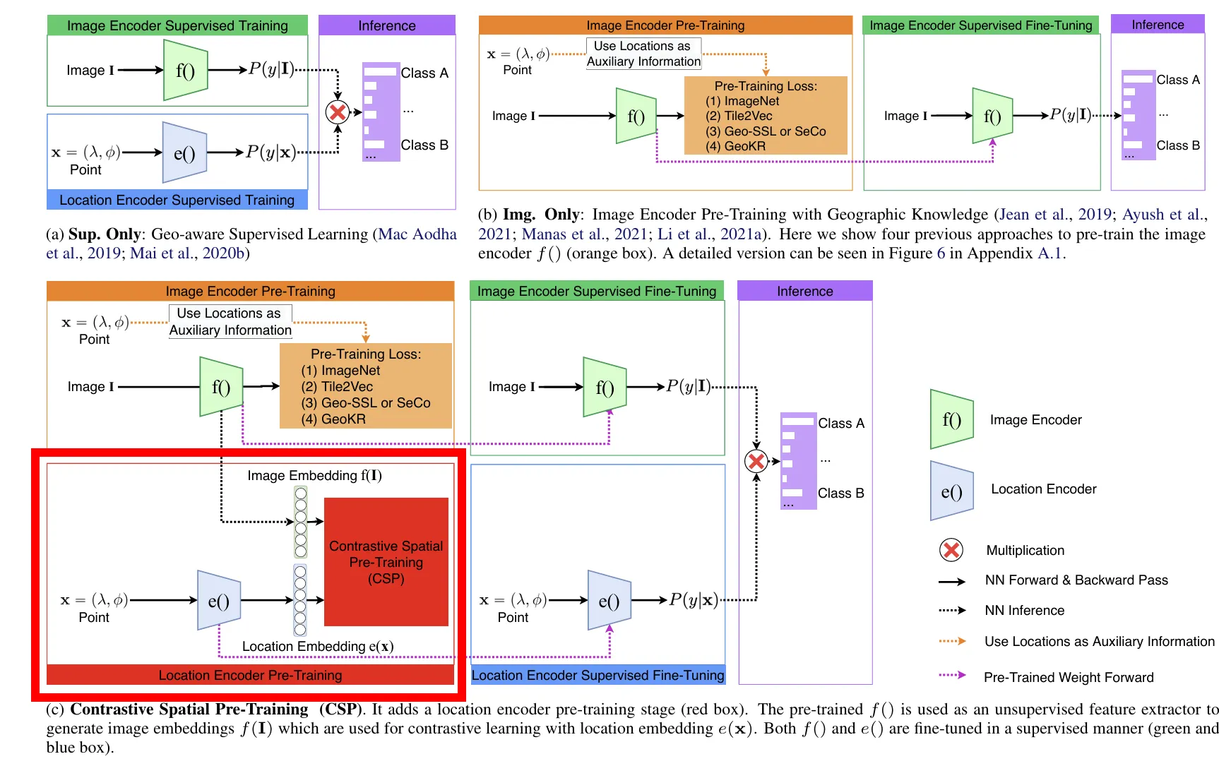
CSP proposes a two-stage training pipeline:
1.
Contrastive Spatial Pre-Training: A label-free self-supervised learning phase that aligns location encoder e(x) and image encoder f(I) in a geospatially aligned representation space.
2.
Supervised Fine-Tuning: Task-specific fine-tuning with labeled data to optimize for downstream applications.
The fundamental goal of the pre-training phase is to learn representations where geographically proximate images are embedded close to their corresponding location encodings in the shared latent space.
Architecture Overview
Location Encoder
The LocationEncoder module serves as the core component for encoding geographic coordinates into meaningful embeddings. Key features include:
•
Spatial Encoder Integration: Uses a spatial encoder (spa_enc) to transform 2D location coordinates into high-dimensional embeddings
•
Classification Head: Includes a linear layer for multi-class prediction
•
Flexible Output: Can return either raw location embeddings or class predictions depending on the use case
The forward pass converts location coordinates (batch_size, 2) into spatial embeddings (batch_size, num_filts) through the spatial encoder, which can then be used for downstream tasks.
class LocationEncoder(nn.Module):
def __init__(self, spa_enc, num_inputs, num_classes, num_filts, num_users=1):
'''
Args:
spa_enc: the spatial encoder
num_inputs: input embedding dimention
num_classes: number of categories we want to classify
num_filts: hidden embedding dimention
'''
super(LocationEncoder, self).__init__()
self.spa_enc = spa_enc
self.inc_bias = False
self.num_filts = num_filts
self.num_classes = num_classes
self.num_users = num_users
self.class_emb = nn.Linear(num_filts, num_classes, bias=self.inc_bias)
self.user_emb = nn.Linear(num_filts, num_users, bias=self.inc_bias)
def forward(self, x, class_of_interest=None, return_feats=False):
'''
Args:
x: torch.FloatTensor(), input location features (batch_size, input_loc_dim = 2)
class_of_interest: the class id we want to extract
return_feats: whether or not just return location embedding
'''
# loc_feat: (batch_size, 1, input_loc_dim = 2)
loc_feat = torch.unsqueeze(x, dim=1)
loc_feat = loc_feat.cpu().data.numpy()
# loc_embed: torch.Tensor(), (batch_size, 1, spa_embed_dim = num_filts)
loc_embed = self.spa_enc(loc_feat)
# loc_emb: torch.Tensor(), (batch_size, spa_embed_dim = num_filts)
loc_emb = loc_embed.squeeze(1)
if return_feats:
# loc_emb: (batch_size, num_filts)
return loc_emb
if class_of_interest is None:
# class_pred: (batch_size, num_classes)
class_pred = self.class_emb(loc_emb)
else:
# class_pred: shape (batch_size)
class_pred = self.eval_single_class(loc_emb, class_of_interest)
return torch.sigmoid(class_pred)
def eval_single_class(self, x, class_of_interest):
'''
Args:
x: (batch_size, num_filts)
Return:
shape (batch_size)
'''
# note: self.class_emb.weight shape (num_classes, num_filts)
if self.inc_bias:
return torch.matmul(x, self.class_emb.weight[class_of_interest, :]) + self.class_emb.bias[class_of_interest]
else:
return torch.matmul(x, self.class_emb.weight[class_of_interest, :])
Python
복사
Location-Image Encoder
The LocationImageEncoder extends the location encoder by incorporating image features and supporting various self-supervised loss functions. This architecture enables:
•
Joint Location-Image Representation: Combines location embeddings with CNN-extracted image features
•
Multiple Loss Functions: Supports L2 regression loss, image contrastive loss, and continuous softmax loss
•
Projection Layers: Includes optional decoder layers for different self-supervised learning objectives
•
◦
Rethinking the inception architecture for computer vision. In Proceedings of the IEEE conference on computer vision and pattern recognition, pp. 2818–2826, 2016.
class LocationImageEncoder(nn.Module):
def __init__(self, loc_enc, train_loss, unsuper_loss = "none", cnn_feat_dim = 2048, spa_enc_type = "gridcell"):
'''
Args:
loc_enc: LocationEncoder() or FCNet()
'''
super(LocationImageEncoder, self).__init__()
self.loc_enc = loc_enc
if spa_enc_type in ["geo_net"]:
self.spa_enc = loc_enc
else:
self.spa_enc = loc_enc.spa_enc
self.inc_bias = loc_enc.inc_bias
self.class_emb = loc_enc.class_emb
self.user_emb = loc_enc.user_emb
self.cnn_feat_dim = cnn_feat_dim
self.loc_emb_dim = loc_enc.num_filts
if unsuper_loss == "none":
return
elif unsuper_loss == "l2regress":
self.loc_dec = nn.Linear(in_features = self.loc_emb_dim, out_features = self.cnn_feat_dim, bias = True)
elif "imgcontloss" in unsuper_loss or "contsoftmax" in unsuper_loss:
self.img_dec = nn.Linear(in_features = self.cnn_feat_dim, out_features = self.loc_emb_dim, bias = True)
else:
raise Exception(f"Unknown unsuper_loss={unsuper_loss}")
def forward(self, x, class_of_interest=None, return_feats=False):
'''
Args:
x: torch.FloatTensor(), input location features (batch_size, input_loc_dim = 2)
class_of_interest: the class id we want to extract
return_feats: whether or not just return location embedding
'''
return self.loc_enc.forward(x, class_of_interest, return_feats)
def eval_single_class(self, x, class_of_interest):
'''
Args:
x: (batch_size, num_filts)
Return:
shape (batch_size)
'''
return self.loc_enc.eval_single_class(x, class_of_interest)
Python
복사
Contrastive Learning Strategy
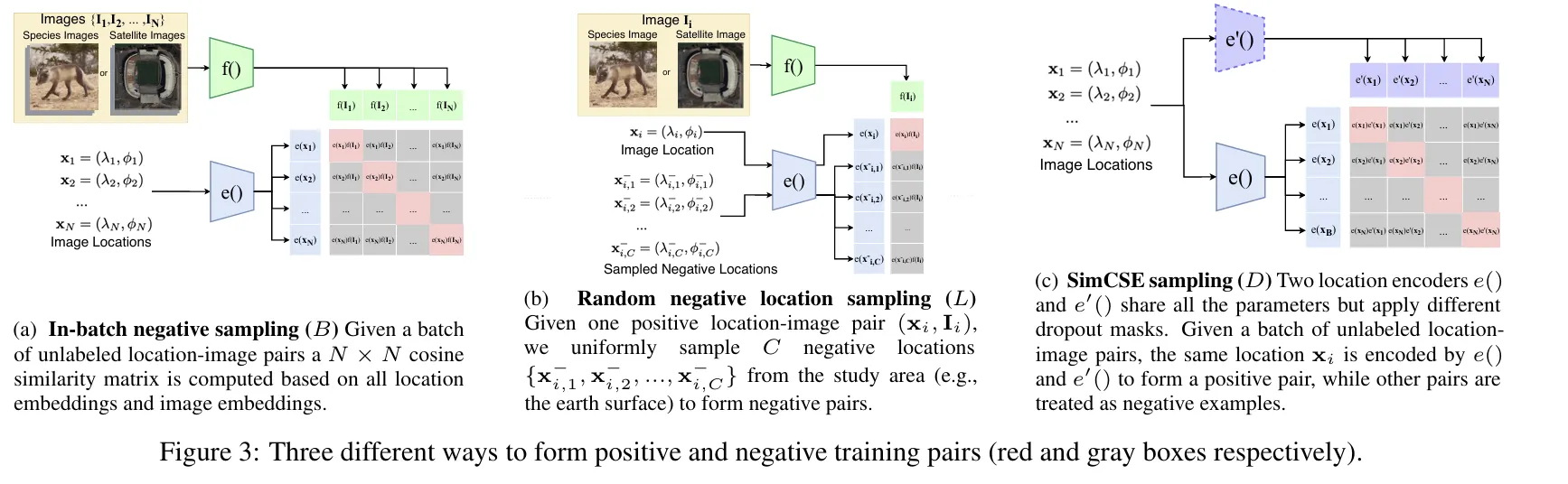
The paper explores three distinct approaches for constructing positive and negative pairs during pre-training:
① In-Batch Negative Sampling
Uses other samples within the same batch as negative examples. This is computationally efficient but may suffer from false negatives when batch samples are geographically close.
Definition
Given a mini-batch of location-image pairs, each anchor pair uses all other samples in the batch as negatives.
•
Positive:
•
Negatives:
This provides a set of contrastive negatives entirely from the current batch.
Loss Formulation
The denominator contains all batch locations, so the model must distinguish the correct location embedding from all others in the batch.
② Random Negative Location Sampling
Randomly samples geographic locations as negatives, ensuring greater diversity in negative examples and reducing the likelihood of false negatives.
Definition
Instead of using only in-batch negatives, this method draws random geographic locations from the whole spatial distribution.
The image is fixed, but its paired location is replaced by randomly sampled negatives.
•
Positive:
•
Negatives: randomly sampled locations paired with the same image
This increases the diversity of negative examples and reduces false negatives.
Loss Formulation
Where
are independently sampled negative locations.
③ SimCSE-Style Location Positive Augmentation
Creates positive pairs by augmenting the same location with slight perturbations, inspired by SimCSE's approach in NLP. This helps the model learn robust location representations invariant to small spatial variation 수식anchor = (e(x_i))positive = (e'(x_i))[
수식anchor = (e(x_i))positive = (e'(x_i))[Definition
Inspired by SimCSE in NLP, the same location is encoded twice with different dropout masks or encoder stochasticity.
These two embeddings form a positive pair, enforcing invariance to small perturbations.
•
Positive: two different encodings of the same location
•
Negatives: other locations in the batch
Loss Formulation
The encoder is trained to produce consistent representations for the same location while separating it from all other locations in the batch.
Loss Functions
The paper evaluates three self-supervised loss functions:
NCE (Noise Contrastive Estimation) Loss
A standard contrastive loss that encourages positive pairs to have similar embeddings while pushing negative pairs apart.
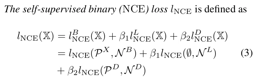
MC (InfoNCE-style Multi-Class) Loss
A multi-class variant of the InfoNCE loss that treats each negative sample as a separate class. This approach achieved the best performance in the paper's experiments, demonstrating superior ability to learn discriminative geospatial representations.
L2/MSE Regression Loss
Attempts to directly regress location embeddings to image features using mean squared error. However, this approach showed poor performance compared to contrastive methods.
Training Methodology
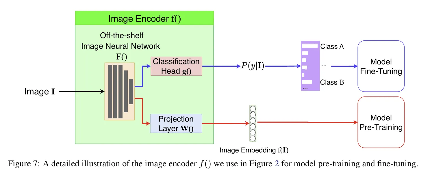
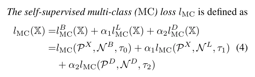
Image Encoder Pre-Training
Following insights from the LiT (Locked-image Tuning) paper, CSP adopts a two-phase approach:
1.
Pre-train the image encoder f(I) first
2.
Lock the image encoder and use it to pre-train the location encoder e(x) (Self-Supervised Fine Tuning)
During CSP pre-training, only the image projection layer W() is trained while the rest of the image encoder remains frozen. This strategy significantly improves performance by preventing the image encoder from overfitting to the specific geospatial task.
Drop
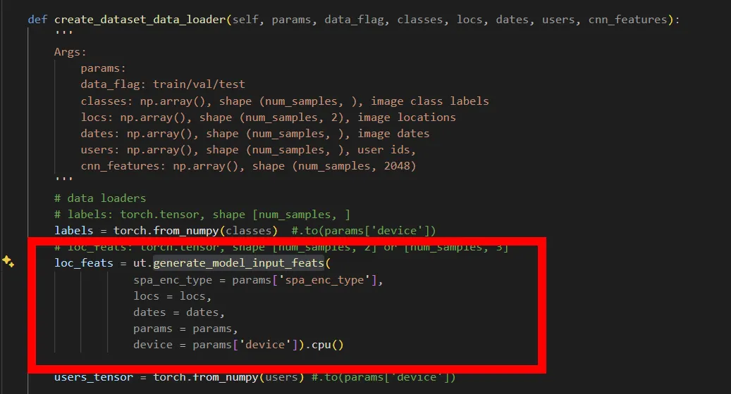
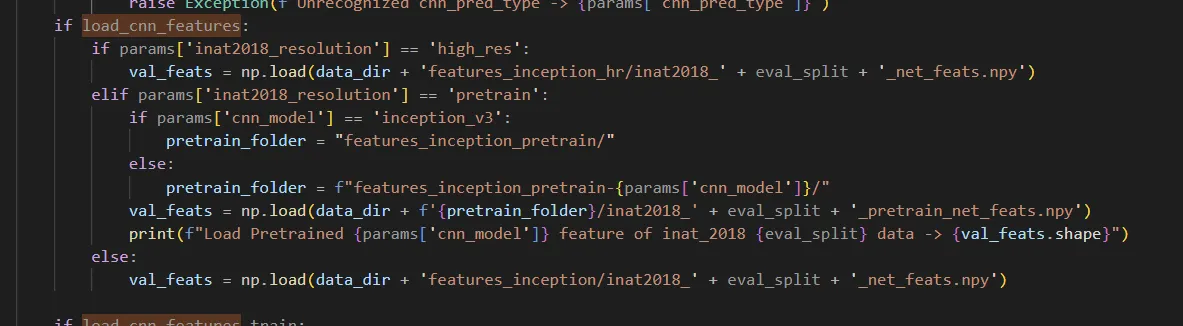
Feature Extraction Pipeline
The implementation shows that:
•
Location features are extracted dynamically during data loading
•
CNN image features appear to be pre-computed and stored in the preprocessed dataset
•
The spatial encoder transforms raw coordinates into embeddings suitable for contrastive learning
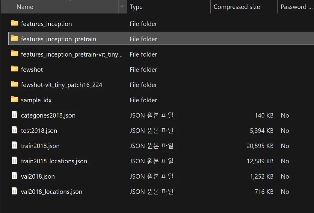
Prior Dataset
Key Insights and Contributions
•
Self-Supervised Geospatial Learning: Demonstrates that contrastive learning can effectively align visual and spatial modalities without requiring labeled data
•
MC Loss Superiority: Shows that InfoNCE-style multi-class loss outperforms other contrastive objectives for this task
•
Locked Image Encoder: Validates that freezing the image encoder during location encoder pre-training improves generalization
•
Flexible Architecture: The modular design allows easy integration of different spatial encoders and loss functions
Conclusion
CSP presents a well-designed framework for learning geospatially aligned visual representations through self-supervised contrastive learning. By carefully designing positive/negative pair construction strategies and selecting appropriate loss functions, the paper demonstrates significant improvements in geospatial-visual tasks. The locked image encoder strategy and the superiority of MC loss provide valuable insights for future multimodal geospatial learning research.
The clean separation between pre-training and fine-tuning phases, combined with the modular architecture, makes this approach both theoretically sound and practically applicable to various geospatial computer vision tasks.
Appendix
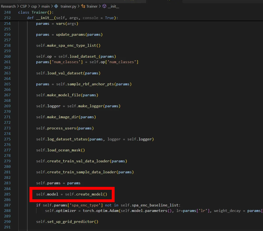
•
The code generates models and input features when loading data