
•
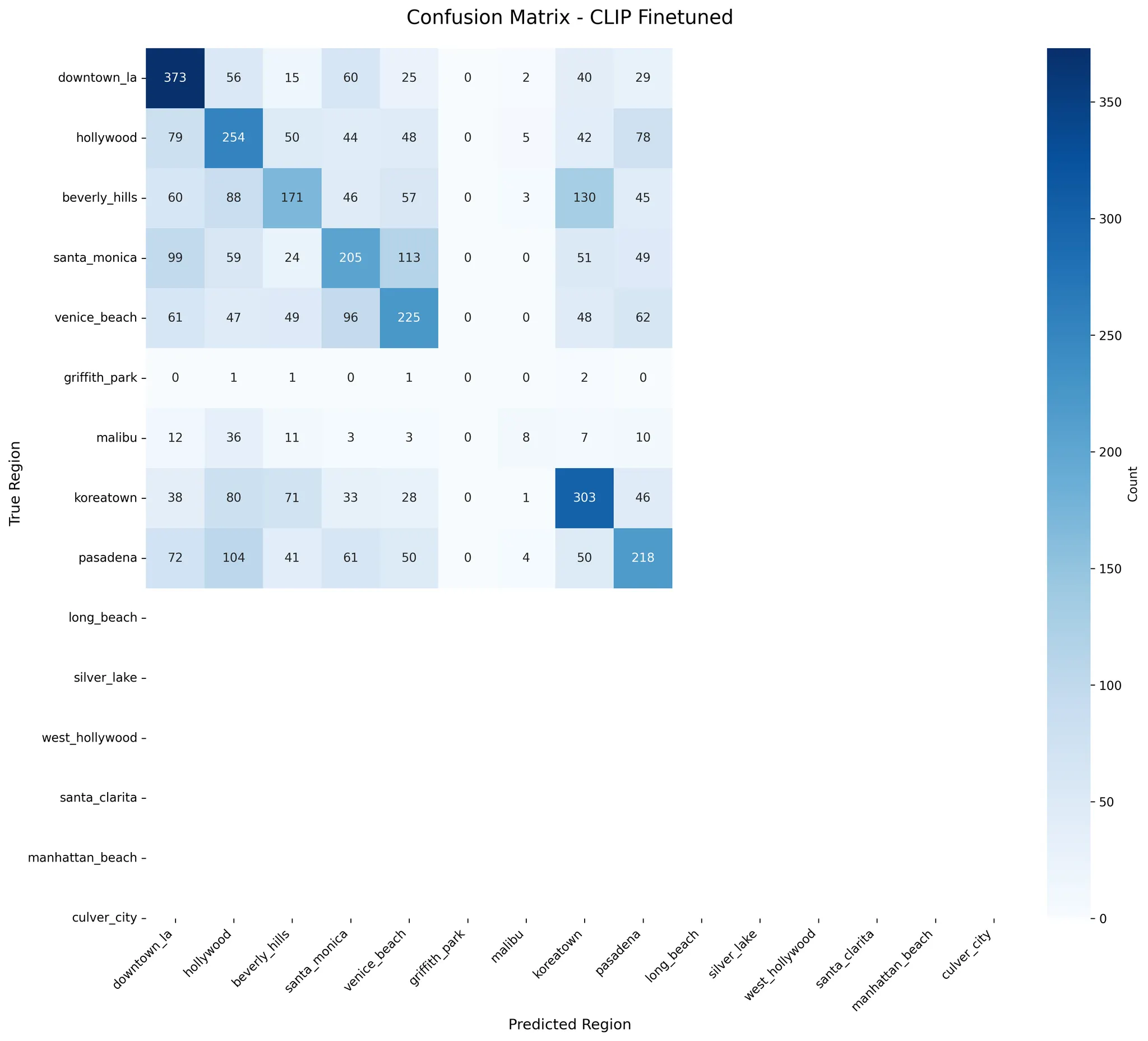
Fine-tuned CLIP ViT-32 model improved accuracy from 0.14 to 0.41 on LA County sub-city level geolocation task after 8 epochs of training
•
Dataset consists of 28,551 images across 9 regions for training, with 15 regions tested during inference
•
Model uses CLIP's vision-language matching: compares image embeddings against region text embeddings (e.g., "A street view photo from Downtown Los Angeles, LA's financial and cultural center - skyline")
•
Prediction method: calculates cosine similarity between normalized image and text embeddings, applies softmax for probability distribution, returns top-k region centroids as GPS coordinates
•
Performance metrics on 5000 sampled images: ACC@1km: 9.78%, ACC@5km: 15.32%, ACC@10km: 27.86%
•
Venice Beach achieved highest recall (0.26) among regions, while Long Beach showed highest precision (0.87) in initial CLIP evaluation
•
Zero-shot classification approach maps predicted regions to their bounding box centroids for GPS coordinate estimation
Comparision of Finetuned CLIP and in Sub-city Level
Overview
•
Data Collection
◦
Total 28551 imgs → sampled approximately 6800 imgs
◦
Examples


Finetuning CLIP
•
Target: CLIP ViT-32
◦
Training was stopped at 8 epochs (Best Evaluation)

After Finetuning,
Accuracy was improved on test dataset 0.14 → 0.41
After Finetuning (Because of Data Collection was stopped)
Before Finetuning
# LA County Geolocation Experiment Report
Date: 2026-01-04 19:13:51
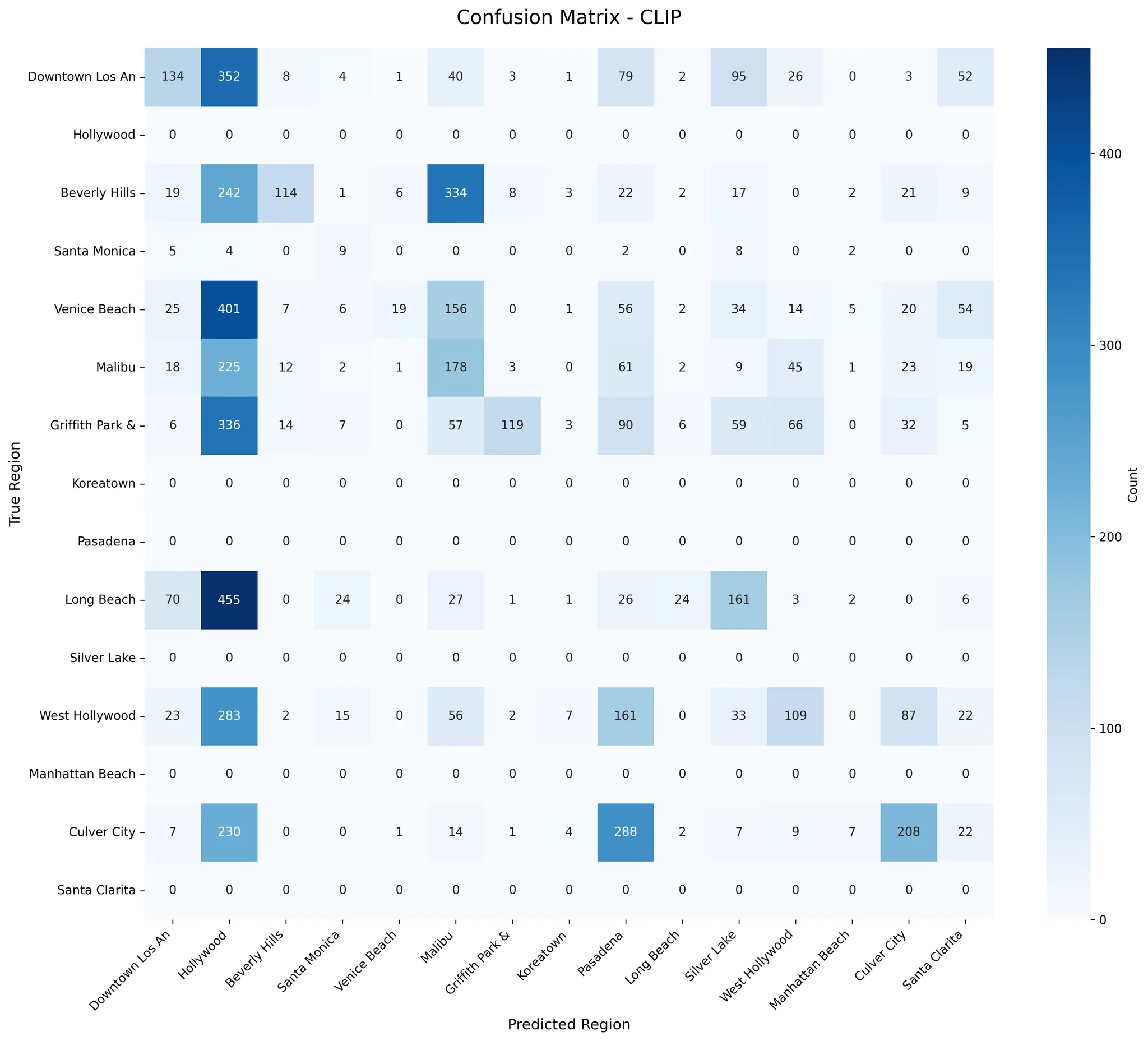
## Model Performance Comparison
| Model | Accuracy | Precision | Recall | F1 Score |
|:--------|-----------:|------------:|---------:|-----------:|
| CLIP | 0.147 | 0.565 | 0.147 | 0.203 |
## CLIP Detailed Results
- **Accuracy**: 0.147
- **Precision**: 0.565
- **Recall**: 0.147
- **F1 Score**: 0.203
### Per-Region Performance
```
precision recall f1-score support
Downtown Los Angeles 0.73 0.14 0.24 800
Hollywood 0.68 0.02 0.05 800
Beverly Hills 0.44 0.17 0.24 800
Santa Monica 0.40 0.14 0.20 800
Venice Beach 0.53 0.26 0.35 800
Malibu 0.00 0.00 0.00 0
Griffith Park & Observatory 0.13 0.30 0.18 30
Koreatown 0.21 0.30 0.24 599
Pasadena 0.60 0.03 0.06 800
Long Beach 0.87 0.15 0.25 800
Silver Lake 0.00 0.00 0.00 0
West Hollywood 0.00 0.00 0.00 0
Manhattan Beach 0.00 0.00 0.00 0
Culver City 0.00 0.00 0.00 0
Santa Clarita 0.00 0.00 0.00 0
accuracy 0.15 6229
macro avg 0.31 0.10 0.12 6229
weighted avg 0.56 0.15 0.20 6229
```
Markdown
복사

Experiment

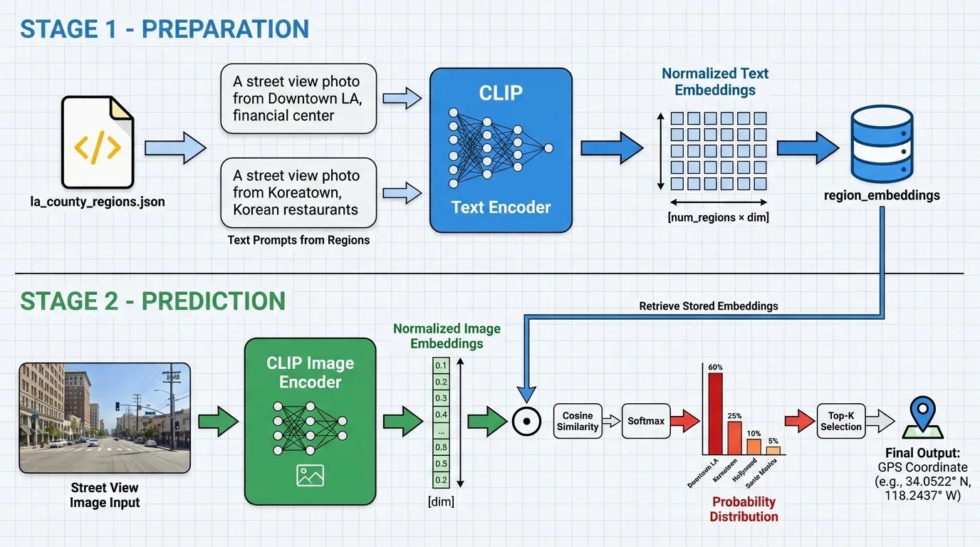
1-1. Preparation Stage: Region Text Embeddings
The constructor first loads region information and creates text embeddings.
self.regions = self._load_regions() # Read la_county_regions.json
self.region_names =list(self.regions.keys())
self._create_region_embeddings()
Python
복사
_create_region_embeddings():
texts = [f"A street view photo from {name}, {info['description']}"
for name, info in self.regions.items()]
inputs =self.processor(text=texts, return_tensors="pt", padding=True).to(self.device)
with torch.no_grad():
text_features =self.model.get_text_features(**inputs)
self.region_embeddings = text_features / text_features.norm(dim=-1, keepdim=True)
Python
복사
For each class, prompts like this are used:
"A street view photo from Downtown Los Angeles, LA's financial and cultural center - skyline, downtown streets"
→ Normalized CLIP text embeddings for these texts are stored in self.region_embeddings. (shape: [num_regions, dim])
1-2. Actual Prediction Flow
predict(self, image_path, top_k=5):
image = Image.open(image_path).convert("RGB")
inputs = self.processor(images=image, return_tensors="pt").to(self.device)
with torch.no_grad():
image_features = self.model.get_image_features(**inputs)
image_features = image_features / image_features.norm(dim=-1, keepdim=True)
Python
복사
1.
Load the image and preprocess with CLIP processor
2.
Extract image embeddings with get_image_features (including normalization)
similarity = (image_features @self.region_embeddings.T).squeeze()
probs = torch.softmax(similarity, dim=0)
Python
복사
3.
Calculate cosine similarity between image embeddings and pre-computed region text embeddings
(Since both are ℓ2 normalized, dot product = cosine similarity)
4.
Apply softmax to the similarity scores → probability distribution over each region
top_probs, top_indices = torch.topk(probs, min(top_k, len(self.region_names)))
top_pred_gps = []
top_pred_prob = []
for idx, prob in zip(top_indices, top_probs):
region_name = self.region_names[idx.item()]
centroid = self.regions[region_name]["centroid"]
top_pred_gps.append(centroid)
top_pred_prob.append(prob.item())
Python
복사
5.
Extract top_k region indices ordered by probability
→ Find the region names
→ Retrieve the region's bbox centroid (latitude, longitude) from la_county_regions.json
Final return value:
return top_pred_gps, top_pred_prob
# Example
top_pred_gps = [(34.05, -118.25), (34.07, -118.30), (34.02, -118.50), ...]
top_pred_prob = [0.62, 0.21, 0.08, ...]
Python
복사
In summary, this is a CLIP zero-shot classification → using region centroids as GPS coordinates approach.
Sampled 5000 images from approximately 8000 data points
Class Examples:
•
"A street view photo from Downtown Los Angeles, LA's financial and cultural center - skyline"
•
"A street view photo from Koreatown, Korean town - Korean restaurants, karaoke"

Result


•
Fine-Tuned CLIP
◦
ACC@1km: 9.78% → Worse than unfinetuned CLIPs
◦
ACC@5km: 15.32%
◦
ACC@10km: 27.86%
