
•
Neural networks learn hierarchical representations through multiple layers of linear transformations followed by nonlinear activation functions, enabling them to approximate complex decision boundaries
•
Common activation functions include ReLU (most widely used), Sigmoid, Tanh, Leaky ReLU, and Swish, each with distinct properties and trade-offs
•
Training neural networks requires computing gradients of the loss function with respect to all parameters using the chain rule
•
Backpropagation efficiently computes all gradients in one forward pass and one backward pass by reusing intermediate computations
•
The backpropagation algorithm consists of: forward pass (compute activations), output layer error computation, backward pass (propagate errors), gradient computation, and parameter updates
•
SGD (Stochastic Gradient Descent) updates parameters using gradients from mini-batches rather than the entire dataset, making training faster and more practical
•
Key challenges include vanishing gradients (mitigated by ReLU), exploding gradients (addressed by gradient clipping and normalization), and memory requirements
•
Modern deep learning frameworks implement automatic differentiation, automating backpropagation for arbitrary computational graphs

Neural Nets & CNN
Neural Nets
Definition
•
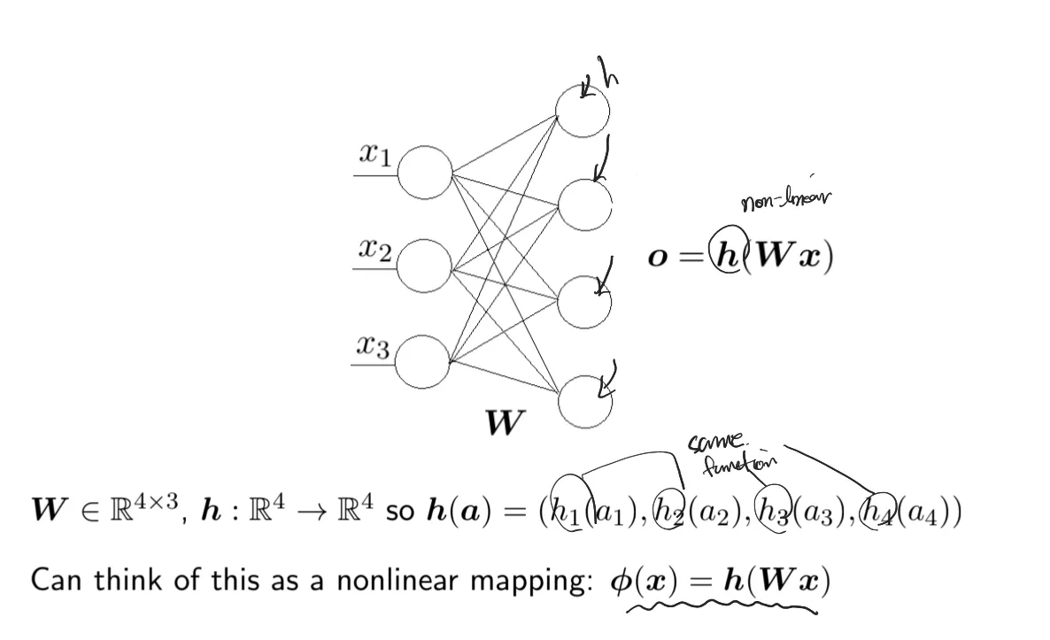
Linear models are not always adequate

How about learning this nonlinear mapping from data?
Instead of hand-crafting features, neural networks can learn hierarchical representations automatically through multiple layers of transformation.
The key idea is to stack multiple layers of linear transformations followed by nonlinear activation functions, allowing the model to approximate complex decision boundaries.

◦
ReLU (Rectified Linear Unit): f(x) = max(0, x)
Most commonly used activation function in deep learning. Computationally efficient and helps mitigate the vanishing gradient problem. However, can suffer from "dying ReLU" problem where neurons can become inactive.
◦
Sigmoid: f(x) = 1 / (1 + e^(-x))
Outputs values between 0 and 1, making it useful for binary classification. However, suffers from vanishing gradient problem for very high or low input values, which can slow down learning in deep networks.
◦
Tanh (Hyperbolic Tangent): f(x) = (e^x - e^(-x)) / (e^x + e^(-x))
Outputs values between -1 and 1, zero-centered unlike sigmoid. Still suffers from vanishing gradient problem but generally performs better than sigmoid in hidden layers.
◦
Leaky ReLU: f(x) = max(αx, x) where α is a small constant (e.g., 0.01)
Addresses the dying ReLU problem by allowing small negative values when x < 0. Maintains most benefits of ReLU while preventing neuron death.
◦
Swish: f(x) = x · sigmoid(x)
Developed by Google, this smooth, non-monotonic function has been shown to outperform ReLU on deeper models. Self-gated and computationally efficient.
•
Each node is called a neuron
•
is called the activation function
•
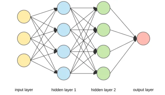
The number of layers refers to the number of hidden layers and Deep Neural Nets can have many layers and millions of parameters
•
This is a feedforward, fully connected neural net and there are many variants.
•
Math Formulation

Our Goal is to minimize the loss function

Let’s calculate the gradient of this complicated function
◦
We need Chain Rule only

To train the neural network, we need to compute gradients of the loss function with respect to all parameters. The chain rule allows us to efficiently compute these gradients through backpropagation.
First, compute all activations layer by layer during the forward pass. Then, starting from the output layer, compute gradients by applying the chain rule during the backward pass (backpropagation).
For the output layer, compute the gradient of the loss with respect to the output layer weights: ∂L/∂W₃ = ∂L/∂y · ∂y/∂W₃
For each hidden layer, propagate the gradient backward: ∂L/∂W₂ = ∂L/∂h₂ · ∂h₂/∂W₂ and ∂L/∂W₁ = ∂L/∂h₁ · ∂h₁/∂W₁, where each ∂L/∂h is computed by chaining through the subsequent layers.
At each layer, multiply by the derivative of the activation function: ∂L/∂z = ∂L/∂h(z) · h'(z). For ReLU: h'(z) = 1 if z > 0, else 0. For Sigmoid: h'(z) = h(z)(1 - h(z)).
Once gradients are computed, update parameters using gradient descent: W ← W - η · ∂L/∂W, where η is the learning rate.

Let's derive the gradient computation step by step. Consider a simple neural network with input x, hidden layer h, and output y. The forward pass computes:
z₁ = W₁x + b₁
h = σ(z₁)
z₂ = W₂h + b₂
y = σ(z₂)
where σ denotes the activation function. For a loss function L(y, t) where t is the target, we want to compute ∂L/∂W₁, ∂L/∂b₁, ∂L/∂W₂, and ∂L/∂b₂.
Step 1: Gradient with respect to output layer parameters
First, compute the gradient of the loss with respect to the pre-activation output:
∂L/∂z₂ = ∂L/∂y · ∂y/∂z₂ = ∂L/∂y · σ'(z₂)
Then, the gradient with respect to W₂ and b₂:
∂L/∂W₂ = ∂L/∂z₂ · ∂z₂/∂W₂ = ∂L/∂z₂ · hᵀ
∂L/∂b₂ = ∂L/∂z₂
Let δ₂ = ∂L/∂z₂ for convenience.
Step 2: Backpropagate to hidden layer
To compute gradients for the hidden layer, we need ∂L/∂h:
∂L/∂h = ∂L/∂z₂ · ∂z₂/∂h = δ₂ · W₂ᵀ
Then compute the gradient with respect to the pre-activation hidden layer:
∂L/∂z₁ = ∂L/∂h · ∂h/∂z₁ = (δ₂ · W₂ᵀ) ⊙ σ'(z₁)
where ⊙ denotes element-wise multiplication. Let δ₁ = ∂L/∂z₁.
Step 3: Gradient with respect to input layer parameters
Finally, compute gradients for W₁ and b₁:
∂L/∂W₁ = ∂L/∂z₁ · ∂z₁/∂W₁ = δ₁ · xᵀ
∂L/∂b₁ = δ₁
General pattern for layer l
For a general layer l, the backpropagation algorithm computes:
δₗ = (Wₗ₊₁ᵀ · δₗ₊₁) ⊙ σ'(zₗ)
∂L/∂Wₗ = δₗ · aₗ₋₁ᵀ
∂L/∂bₗ = δₗ
where aₗ₋₁ is the activation from the previous layer. This recursive formula allows us to efficiently compute gradients for all layers by propagating error terms backward through the network.


Backpropagation

Backpropagation Algorithm
Backpropagation is the fundamental algorithm for training neural networks. It efficiently computes the gradient of the loss function with respect to each parameter in the network by applying the chain rule of calculus in reverse order, from output to input layers.
Why Backpropagation?
Computing gradients naively for each parameter would require separate forward passes through the network, making training computationally prohibitive. Backpropagation solves this by reusing intermediate computations, calculating all gradients in just one forward pass and one backward pass.
The Algorithm Steps
1.
Forward Pass: Compute and store all activations
Starting from the input layer, compute the output of each layer sequentially:
z⁽ˡ⁾ = W⁽ˡ⁾a⁽ˡ⁻¹⁾ + b⁽ˡ⁾
a⁽ˡ⁾ = σ(z⁽ˡ⁾)
where l denotes the layer number, z⁽ˡ⁾ is the pre-activation, a⁽ˡ⁾ is the activation, W⁽ˡ⁾ and b⁽ˡ⁾ are the weights and biases, and σ is the activation function.
Store all intermediate values (z⁽ˡ⁾ and a⁽ˡ⁾) as they will be needed in the backward pass.
2.
Compute Output Layer Error: Calculate the gradient at the output
For the output layer L, compute the error term (delta):
δ⁽ᴸ⁾ = ∂L/∂z⁽ᴸ⁾ = ∂L/∂a⁽ᴸ⁾ ⊙ σ'(z⁽ᴸ⁾)
For common loss functions:
•
Mean Squared Error with linear output: δ⁽ᴸ⁾ = a⁽ᴸ⁾ - y
•
Cross-Entropy with softmax: δ⁽ᴸ⁾ = a⁽ᴸ⁾ - y
where y is the target output.
3.
Backward Pass: Propagate error backward through layers
For each layer l = L-1, L-2, ..., 1, compute the error term by propagating the error from layer l+1:
δ⁽ˡ⁾ = (W⁽ˡ⁺¹⁾)ᵀ δ⁽ˡ⁺¹⁾ ⊙ σ'(z⁽ˡ⁾)
This step applies the chain rule: the gradient at layer l depends on the gradient at layer l+1 multiplied (backpropagated) through the weights, then element-wise multiplied by the derivative of the activation function.
The ⊙ symbol denotes element-wise (Hadamard) multiplication.
4.
Compute Parameter Gradients: Calculate gradients for weights and biases
Once we have the error terms δ⁽ˡ⁾ for all layers, compute the gradients:
∂L/∂W⁽ˡ⁾ = δ⁽ˡ⁾ (a⁽ˡ⁻¹⁾)ᵀ
∂L/∂b⁽ˡ⁾ = δ⁽ˡ⁾
For mini-batch training, these gradients are averaged over all examples in the batch.
5.
Update Parameters: Apply gradient descent
Update all weights and biases using the computed gradients:
W⁽ˡ⁾ ← W⁽ˡ⁾ - η · ∂L/∂W⁽ˡ⁾
b⁽ˡ⁾ ← b⁽ˡ⁾ - η · ∂L/∂b⁽ˡ⁾
where η is the learning rate.
Key Insights
•
Chain Rule Application: Backpropagation systematically applies the chain rule to compute how changes in each parameter affect the final loss
•
Computational Efficiency: By storing forward pass results and reusing them during the backward pass, we compute all gradients in O(1) time relative to computing them independently
•
Modularity: Each layer only needs to know how to compute its own forward pass and the gradient of its activation function. The algorithm works for any network architecture
•
Automatic Differentiation: Modern deep learning frameworks (PyTorch, TensorFlow) implement automatic differentiation, which automates backpropagation for arbitrary computational graphs
Activation Function Derivatives
The derivative of the activation function σ'(z) is crucial for backpropagation:
•
ReLU: σ'(z) = 1 if z > 0, else 0
•
Sigmoid: σ'(z) = σ(z)(1 - σ(z))
•
Tanh: σ'(z) = 1 - tanh²(z)
•
Leaky ReLU: σ'(z) = 1 if z > 0, else α
Practical Considerations
•
Vanishing Gradients: When using sigmoid or tanh activations in deep networks, gradients can become very small as they propagate backward, making training slow or ineffective. ReLU helps mitigate this.
•
Exploding Gradients: Gradients can grow exponentially in deep networks. Solutions include gradient clipping, careful weight initialization, and batch normalization.
•
Memory Requirements: Backpropagation requires storing all forward pass activations, which can be memory-intensive for deep networks. Techniques like gradient checkpointing trade computation for memory.
Simple Example
Consider a network with one hidden layer: x → h → y
Forward pass:
z₁ = W₁x + b₁
h = ReLU(z₁)
z₂ = W₂h + b₂
y = σ(z₂)
L = (y - t)²
Backward pass:
∂L/∂y = 2(y - t)
δ₂ = ∂L/∂z₂ = ∂L/∂y · σ'(z₂) = 2(y - t) · σ(z₂)(1 - σ(z₂))
∂L/∂W₂ = δ₂ · hᵀ
∂L/∂b₂ = δ₂
∂L/∂h = W₂ᵀ · δ₂
δ₁ = ∂L/∂h ⊙ ReLU'(z₁) where ReLU'(z₁) = 1 if z₁ > 0, else 0
∂L/∂W₁ = δ₁ · xᵀ
∂L/∂b₁ = δ₁
Otherwise, we can use SGD for backpropagation

Stochastic Gradient Descent (SGD) is an optimization algorithm that updates model parameters using gradients computed by backpropagation. While standard gradient descent computes gradients using the entire dataset, SGD updates parameters using gradients from individual examples or small mini-batches, making training much faster and more practical for large datasets.
How SGD Works with Backpropagation
The combination of backpropagation and SGD forms the foundation of modern neural network training:
1.
Initialize Parameters: Start with random weights and biases
Initialize all weights W⁽ˡ⁾ and biases b⁽ˡ⁾ with small random values (e.g., from a normal distribution with mean 0 and small variance).
2.
Sample Mini-batch: Randomly select a small batch of training examples
Instead of using the entire dataset, randomly sample a mini-batch of size m (typically 32, 64, 128, or 256 examples). This introduces stochasticity into the optimization process.
3.
Forward Pass: Compute predictions for the mini-batch
For each example in the mini-batch, perform a forward pass through the network to compute predictions and store intermediate activations.
4.
Compute Loss: Calculate the average loss over the mini-batch
Compute the loss function for each example and average across the mini-batch:
L = (1/m) Σᵢ L(ŷᵢ, yᵢ)
where ŷᵢ is the predicted output and yᵢ is the true label for example i.
5.
Backward Pass: Run backpropagation to compute gradients
Apply the backpropagation algorithm to compute gradients of the loss with respect to all parameters, averaged over the mini-batch:
∂L/∂W⁽ˡ⁾ = (1/m) Σᵢ ∂Lᵢ/∂W⁽ˡ⁾
∂L/∂b⁽ˡ⁾ = (1/m) Σᵢ ∂Lᵢ/∂b⁽ˡ⁾
6.
Update Parameters: Apply SGD update rule
Update all weights and biases using the computed gradients and learning rate η:
W⁽ˡ⁾ ← W⁽ˡ⁾ - η · ∂L/∂W⁽ˡ⁾
b⁽ˡ⁾ ← b⁽ˡ⁾ - η · ∂L/∂b⁽ˡ⁾
7.
Repeat: Continue with next mini-batch
Repeat steps 2-6 for the next mini-batch. One complete pass through all training data is called an epoch. Training typically involves multiple epochs until convergence.
Key Concepts
•
Mini-batch Size: The number of examples used to compute each gradient update
◦
Larger batches: more stable gradients, better hardware utilization, but slower updates
◦
Smaller batches: noisier gradients, faster updates, may help escape local minima, better generalization
◦
Common choices: 32, 64, 128, 256
•
Learning Rate (η): Controls the step size of parameter updates
◦
Too large: training may diverge or oscillate
◦
Too small: training is very slow and may get stuck in local minima
◦
Typical values: 0.001 to 0.1, often requires tuning
◦
Learning rate schedules: gradually decrease learning rate during training (e.g., step decay, exponential decay, cosine annealing)
•
Epoch: One complete pass through the entire training dataset
◦
If dataset has N examples and mini-batch size is m, one epoch contains N/m mini-batch updates
◦
Training typically requires multiple epochs (tens to hundreds)
•
Iteration: One mini-batch gradient update
◦
Number of iterations per epoch = ⌈N/m⌉
SGD Algorithm (Pseudocode)
# Initialize parameters
for each layer l:
W[l] = random_initialization()
b[l] = zeros()
# Training loop
for epoch in range(num_epochs):
# Shuffle training data
shuffle(training_data)
# Iterate through mini-batches
for mini_batch in get_mini_batches(training_data, batch_size):
# Forward pass
activations = forward_pass(mini_batch, W, b)
# Compute loss
loss = compute_loss(activations[-1], mini_batch.labels)
# Backward pass (backpropagation)
gradients = backpropagation(loss, activations, W, b)
# SGD update
for each layer l:
W[l] = W[l] - learning_rate * gradients.dW[l]
b[l] = b[l] - learning_rate * gradients.db[l]
Python
복사
Variants of SGD
•
Batch Gradient Descent: Uses entire dataset for each update
◦
Most stable but very slow for large datasets
◦
Update rule: θ ← θ - η · (1/N) Σᵢ₌₁ᴺ ∂Lᵢ/∂θ
•
Stochastic Gradient Descent (SGD): Uses single example for each update
◦
Fastest updates but very noisy gradients
◦
Update rule: θ ← θ - η · ∂Lᵢ/∂θ
•
Mini-batch SGD: Uses small batch of examples (most common in practice)
◦
Good balance between speed and stability
◦
Update rule: θ ← θ - η · (1/m) Σᵢ∈batch ∂Lᵢ/∂θ
•
SGD with Momentum: Accumulates velocity to accelerate convergence
◦
v ← βv + ∂L/∂θ
◦
θ ← θ - ηv
◦
Momentum coefficient β typically 0.9 or 0.99
◦
Helps overcome small local minima and accelerates training in relevant directions
•
Adam (Adaptive Moment Estimation): Combines momentum with adaptive learning rates
◦
Maintains both first moment (mean) and second moment (variance) of gradients
◦
Automatically adjusts learning rate for each parameter
◦
Most popular optimizer in practice, robust to hyperparameter choices
◦
Default parameters often work well: β₁=0.9, β₂=0.999, ε=10⁻⁸
Preventing Overfitting
What is Overfitting?
Overfitting occurs when a neural network learns the training data too well, including its noise and random fluctuations, rather than learning the underlying patterns that generalize to new, unseen data. An overfitted model performs excellently on training data but poorly on validation/test data.
The model essentially memorizes the training examples instead of learning generalizable features. This happens when:
•
The model is too complex (too many parameters) relative to the amount of training data
•
Training is performed for too many epochs
•
There is insufficient training data
•
The training data is not representative of the real-world distribution
Signs of overfitting include a large gap between training accuracy and validation accuracy, where training loss continues to decrease while validation loss starts increasing.
Methods to Prevent Overfitting
•
Regularization (L1 and L2): Add a penalty term to the loss function that discourages large weights
◦
L2 regularization (weight decay): L_total = L_original + λ Σ(w²)
◦
L1 regularization: L_total = L_original + λ Σ|w|
◦
The hyperparameter λ controls the strength of regularization. L2 regularization encourages small weights, while L1 can drive some weights to exactly zero, performing feature selection.

•
Dropout: During training, randomly "drop" (set to zero) a fraction of neurons in each layer with probability pThis prevents neurons from co-adapting too much and forces the network to learn redundant representations. Dropout acts as an ensemble method, training multiple sub-networks simultaneously.At test time, all neurons are used but their outputs are scaled by (1-p) to account for the increased number of active neurons.Typical dropout rates: 0.2-0.5 for hidden layers, 0.5 being common.

•
Early Stopping: Monitor validation loss during training and stop when it starts increasingKeep track of the model parameters that achieved the best validation performance. This prevents the model from continuing to overfit the training data after it has learned the generalizable patterns.Typically implemented with a patience parameter: stop training if validation loss doesn't improve for N consecutive epochs.

•
Data Augmentation: Artificially increase the size and diversity of the training datasetFor images: random rotations, translations, flips, crops, color jittering, scalingFor text: synonym replacement, back-translation, random insertion/deletionFor audio: time stretching, pitch shifting, adding noiseThis helps the model learn invariant features and improves generalization by exposing it to more diverse examples.

•
Batch Normalization: Normalize layer inputs across the mini-batch
◦
For each mini-batch, normalize the inputs to have mean 0 and variance 1: x_norm = (x - μ_batch) / √(σ²_batch + ε)Then apply learnable scale (γ) and shift (β) parameters: y = γ · x_norm + βBenefits: allows higher learning rates, reduces sensitivity to initialization, acts as regularization, and accelerates training.

•
And many other methods
Convolutional Neural Networks (CNN)
Convolutional Neural Networks (CNNs) are specialized neural networks designed to process grid-like data, particularly images. Unlike standard neural networks that use fully connected layers, CNNs exploit the spatial structure of images through three key operations: convolution, pooling, and local connectivity. This architecture dramatically reduces the number of parameters while maintaining the ability to learn hierarchical features from raw pixel data.
Motivation

Why Standard Neural Networks Don't Work Well for Images
Standard fully connected neural networks face several critical challenges when processing image data:
•
Massive Parameter Count: For a modest 224×224 RGB image, a single fully connected layer with 1000 neurons requires 224×224×3×1000 = 150 million parameters. This leads to computational inefficiency, memory constraints, and severe overfitting.
•
Loss of Spatial Structure: Flattening 2D images into 1D vectors destroys the inherent spatial relationships between pixels. Nearby pixels in an image are highly correlated, but this local structure is completely ignored in fully connected layers.
•
Lack of Translation Invariance: A fully connected network must learn separate features for objects at different positions in the image. If a cat appears in the top-left corner during training but bottom-right during testing, the network may fail to recognize it.
•
No Feature Hierarchy: Standard networks don't naturally build up hierarchical representations from simple edges and textures to complex object parts and whole objects.

CNNs Address These Limitations
Convolutional Neural Networks solve these problems through three fundamental principles that make them ideally suited for visual data:
•
Local Connectivity: Each neuron connects only to a small local region of the input (called the receptive field), drastically reducing parameters while preserving spatial relationships. Instead of connecting every input pixel to every neuron, CNN neurons look at small patches (e.g., 3×3 or 5×5 regions).

Architecture
1.
Convolution Layer

The convolution layer is the core building block of CNNs. It applies a set of learnable filters (also called kernels) to the input, where each filter slides across the spatial dimensions to detect specific features like edges, textures, or patterns.
Key Components:
•
Filter/Kernel: A small matrix (e.g., 3×3, 5×5) of learnable weights that slides over the input
◦
Each filter detects a specific feature across the entire image
◦
Multiple filters are applied in parallel to detect different features
◦
Filter depth must match input depth (e.g., 3 channels for RGB images)
How Convolution Network Works:
The convolution operation is a mathematical operation that slides a filter (kernel) across the input image to produce a feature map. Here's a step-by-step explanation:
•
Step 1: Position the Filter

◦
Place the filter at the top-left corner of the input image (or feature map)
◦
The filter covers a small rectangular region of the input
•
Step 2: Element-wise Multiplication

◦
Multiply each value in the filter with the corresponding value in the overlapping region of the input
◦
For example, if the filter is 3×3 and positioned over a 3×3 region of the input, perform 9 multiplications
•
Step 3: Sum the Products
◦
Add all the products from step 2 together to get a single number
◦
This sum becomes one value in the output feature map
◦
Mathematical formula: output[i,j] = Σₘ Σₙ input[i+m, j+n] × filter[m,n]
•
Step 4: Add Bias
◦
Add a learnable bias term to the sum: output[i,j] = output[i,j] + bias
•
Step 5: Slide the Filter
◦
Move the filter horizontally by the stride amount (typically 1 pixel)
◦
Repeat steps 2-4 to compute the next output value
◦
When reaching the right edge, move down by stride amount and return to the left side
◦
Continue until the entire input has been covered
•
Step 6: Apply Activation Function

◦
Apply a non-linear activation function (e.g., ReLU) to each output value
◦
This introduces non-linearity into the network

Mathematical Example:
Consider a simple 5×5 input image with a 3×3 filter:
# Input (5×5)
input = [[1, 2, 3, 0, 1],
[0, 1, 2, 3, 1],
[3, 0, 1, 2, 3],
[2, 3, 0, 1, 2],
[1, 0, 3, 2, 1]]
# Filter/Kernel (3×3)
filter = [[1, 0, -1],
[1, 0, -1],
[1, 0, -1]]
# Convolution at position (0,0):
output[0,0] = (1×1 + 2×0 + 3×(-1) +
0×1 + 1×0 + 2×(-1) +
3×1 + 0×0 + 1×(-1))
= 1 + 0 - 3 + 0 + 0 - 2 + 3 + 0 - 1
= -2
# Slide filter right by stride=1 and repeat for position (0,1):
output[0,1] = (2×1 + 3×0 + 0×(-1) +
1×1 + 2×0 + 3×(-1) +
0×1 + 1×0 + 2×(-1))
= 2 + 0 + 0 + 1 + 0 - 3 + 0 + 0 - 2
= -2
# Continue for all positions...
Python
복사
Output Size Calculation:


The size of the output feature map depends on the input size, filter size, stride, and padding:
Output Height = ⌊(Input Height - Filter Height + 2×Padding) / Stride⌋ + 1
Output Width = ⌊(Input Width - Filter Width + 2×Padding) / Stride⌋ + 1
For our example: (5 - 3 + 2×0) / 1 + 1 = 3, so the output is 3×3
Key Properties of Convolution:
◦
Parameter Sharing: The same filter weights are used across the entire image, reducing parameters dramatically
◦
Translation Equivariance: If the input shifts, the output shifts by the same amount
◦
Local Connectivity: Each output value depends only on a small local region of the input
◦
Feature Detection: Different filters learn to detect different features (edges, textures, patterns)

In summary,

2.
Pooling Layer

Pooling layers reduce the spatial dimensions of feature maps while retaining the most important information. This operation serves multiple purposes: it reduces computational cost, decreases the number of parameters (helping prevent overfitting), and provides translation invariance by making the network less sensitive to small shifts in input.
Key Components:
•
Max Pooling: Takes the maximum value from each pooling window
◦
Most commonly used pooling method
◦
Captures the strongest activation in each region
◦
Example: For a 2×2 window over values [1, 3, 2, 4], max pooling returns 4
◦
Provides translation invariance - small shifts in features still produce similar outputs
•
Average Pooling: Computes the average of values in each pooling window
◦
Less common than max pooling in hidden layers
◦
Often used in the final layers before classification
◦
Example: For a 2×2 window over values [1, 3, 2, 4], average pooling returns (1+3+2+4)/4 = 2.5
◦
Provides smoother down-sampling compared to max pooling

•
Typical Architecture for CNNs

The typical CNN architecture follows a hierarchical pattern that progressively extracts features and reduces spatial dimensions:
•
Input Layer: The raw image (e.g., 224×224×3 for RGB images)
◦
Height × Width × Channels
◦
RGB images have 3 channels (Red, Green, Blue)
◦
Grayscale images have 1 channel
•
Convolutional Layers (CONV): Extract local features from the input
◦
Early layers detect simple features (edges, corners, textures)
◦
Deeper layers detect complex features (object parts, patterns)
◦
Each CONV layer is typically followed by an activation function (ReLU)
◦
Multiple filters are applied in parallel to create multiple feature maps
•
Pooling Layers (POOL): Reduce spatial dimensions
◦
Usually placed after one or more CONV layers
◦
Max pooling is most common (takes maximum value in each window)
◦
Reduces computation and provides translation invariance
◦
Typical pooling window: 2×2 with stride 2 (reduces dimensions by half)
•
Pattern Repetition: CONV-RELU-POOL blocks repeat multiple times
◦
Each repetition creates deeper, more abstract feature representations
◦
Spatial dimensions decrease while depth (number of channels) increases
◦
Example progression: 224×224×3 → 112×112×64 → 56×56×128 → 28×28×256
•
Fully Connected Layers (FC): Final classification layers
◦
Feature maps are flattened into a 1D vector
◦
One or more FC layers combine features for final decision
◦
Last FC layer outputs class scores (one per class)
◦
Dropout is often applied here to prevent overfitting
•
Output Layer: Final predictions
◦
Softmax activation for multi-class classification
◦
Sigmoid activation for binary classification
◦
Produces probability distribution over classes
Example: Classic CNN Progression
Popular CNN Architectures:
•
LeNet-5 (1998): First successful CNN, used for handwritten digit recognition
•
AlexNet (2012): Won ImageNet competition, popularized deep learning
•
VGGNet (2014): Used small 3×3 filters stacked deeply
•
ResNet (2015): Introduced skip connections for very deep networks (152 layers)
•
Inception/GoogLeNet (2014): Used parallel convolutions of different sizes
•
MobileNet (2017): Efficient architecture for mobile devices
This hierarchical architecture mimics the human visual system, where simple features are combined to recognize increasingly complex patterns, ultimately enabling tasks like image classification, object detection, and semantic segmentation.
List view
Search