
Summary
•
Support Vector Machines (SVMs) maximize the margin between classes by finding a hyperplane that separates data points with the largest possible distance to the nearest examples (support vectors)
•
Soft-margin SVMs introduce slack variables to handle non-separable data, trading off margin size against classification errors through a hyperparameter C
•
The dual formulation expresses SVM optimization in terms of pairwise dot products between data points, enabling the kernel trick for efficient non-linear classification
•
Support vectors are training points with αₙ > 0 that lie on or violate the margin boundary—only these points determine the final decision boundary
•
Decision trees make predictions by recursively applying simple threshold tests on input features, following a path from root to leaf node
•
Tree construction uses greedy splitting: at each node, the algorithm selects the feature and threshold that minimize conditional entropy (maximize information gain)
•
Entropy measures uncertainty in class distributions—pure nodes have entropy 0, while maximally mixed nodes have entropy 1 (for binary classification)
•
Decision trees are interpretable and easy to visualize, but learning optimal structure globally is computationally intractable, requiring greedy top-down construction

Support Vector Machine (SVM)
Linear model with L2 regularized hinge Loss
•
hinge loss
where y ∈ {-1, +1} is the true label and ŷ is the predicted score (w·x + b)
•
Most Commonly used classifcation algorithms before deep learning
•
Works well with kernel trick
•
Strong theoretical guarantees
Intuition
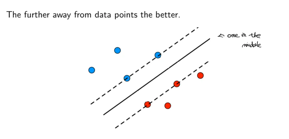
This image illustrates the core intuition behind Support Vector Machines (SVMs).
The blue and red points represent data samples from two different classes. The solid line in the middle is the decision boundary (hyperplane) that separates the two classes, while the two dashed lines indicate the margins. These dashed lines pass through the data points that are closest to the decision boundary, known as support vectors.
The key idea conveyed by the figure is that the farther the decision boundary is from the data points, the better. Rather than choosing any separating line, SVM aims to find the hyperplane that maximizes the margin, i.e., the distance between the decision boundary and the nearest data points from each class.
•
Define Margin; Distance to Hyperplane

This image explains how to compute the distance from a point to a hyperplane, which is fundamental to the definition of the SVM margin.
The hyperplane is defined as . For a given point , the projection onto the hyperplane is assumed to lie along the direction of the normal vetor , scaled by a distance
Starting form the projection assumption:
this leads to:
Therefore, the distance from a point to the hyperplane is given by:
◦
Our goal is to setup a further away hyperplane → Maximized Margins

◦
The margin is defined as the smallest distance from all training points to the hyperplane. Formally, for a classifier parameterized by , the margin is written as:

where is a training point, is its class label, and denotes a feature mapping (possibly nonlinear).
The intuition “the further away, the better” is translated into the following optimization problem:


▪
For a separable training set,
there exists a hyperplane that perfectly separates the two classes with some margin. In this case, all training points satisfy the constraint yₙ(w·φ(xₙ) + b) ≥ 1, and the optimization problem has a feasible solution that achieves the maximum margin.
•
What “seperable” means?
A dataset is called linearly separable if there exists a hyperplane that can perfectly divide the data points of two classes without any errors. In other words, all positive examples lie on one side of the hyperplane and all negative examples lie on the other side, with no overlap or misclassification.
•
Hard Margin
In a hard-margin SVM, we assume that the data is linearly separable and enforce a strict constraint: all training points must lie outside the margin boundaries. This means that every point must satisfy yₙ(w·φ(xₙ) + b) ≥ 1 without exception. While this approach guarantees the maximum possible margin when the data is separable, it is highly sensitive to outliers and noise, making it impractical for real-world datasets where perfect separation is rarely achievable.
▪
But,

•
if data is not linearly separable, the previous constraint is obviously not feasible.
•
Soft-Margin
To address the issue of non-separable data, we introduce slack variables ξₙ ≥ 0 for each training point, which allow some points to violate the margin constraint. The modified optimization problem becomes:

where C is a hyperparameter that controls the trade-off between maximizing the margin and minimizing classification errors. A larger C penalizes margin violations more heavily, resulting in a narrower margin but fewer misclassifications, while a smaller C allows for a wider margin with more tolerance for errors.
◦
SO, Start from the soft-margin SVM formulation

→ we can infer that, at optimality, Slack Variables is
▪
This function is exactly the hinge loss.

▪
NOW, It’s a convex (quadratic in fact) problem
•
→ can apply any convex optimization algorithms, e.g. SGD
•
usually apply kernel trick, which requires soving the dual probledm
Dual Form of SVM
•
What is “Dual From”
The dual form of an optimization problem is an alternative mathematical formulation derived from the original (primal) problem using Lagrangian multipliers. In the context of SVM, the dual form expresses the optimization in terms of the training data points rather than the weight vector w directly. This reformulation is particularly useful because it allows us to apply the kernel trick, enabling SVMs to learn non-linear decision boundaries efficiently without explicitly computing high-dimensional feature mappings.
→ Simply put,
the dual form is a way to rewrite the optimization problem so that it depends on pairwise dot products between data points (⟨φ(xᵢ), φ(xⱼ)⟩) rather than on the weight vector w directly. This makes it possible to use the kernel trick, which allows us to compute these dot products in high-dimensional (or even infinite-dimensional) feature spaces without ever explicitly calculating the feature vectors themselves.

The dual formulation of SVM can be expressed as:
subject to the constraints 0 ≤ αₙ ≤ C and Σαₙyₙ = 0, where αₙ are the Lagrange multipliers. The key advantage of this formulation is that it only depends on the dot products φ(xₙ)ᵀφ(xₘ), which can be replaced by a kernel function K(xₙ, xₘ), enabling efficient computation in high-dimensional feature spaces.
Support Vectors
So, with we induced in the above, what is after we multiply nonlinear function

•
Kernel Trick
The kernel trick is a powerful technique that allows SVMs to efficiently learn non-linear decision boundaries without explicitly computing high-dimensional feature mappings. Instead of transforming data points into a high-dimensional space φ(x) and then computing dot products φ(xᵢ)ᵀφ(xⱼ), we use a kernel function K(xᵢ, xⱼ) = φ(xᵢ)ᵀφ(xⱼ) that directly computes the dot product in the transformed space.
Now we can get very easily with kernel function
•
should be precomputed!!

To sum up, Support vectors are the data points that lie closest to the decision boundary (hyperplane). These points are critical in defining the position and orientation of the hyperplane.
•
Why just consider ?
In the SVM dual formulation, only data points with αₙ > 0 contribute to the decision boundary. These are precisely the support vectors—points that either lie exactly on the margin (yₙ(w·xₙ + b) = 1) or violate it (in the soft-margin case). All other points with αₙ = 0 are correctly classified with sufficient margin and do not influence the hyperplane, making the SVM solution sparse and computationally efficient.
Geometric Interpretation of SVM

This image illustrates the geometric interpretation of support vectors in a Support Vector Machine. A support vector is a training point whose optimal dual variable is greater than zero and satisfies the tight margin condition. Support vectors lie exactly on—or violate—the margin boundary and directly determine the separating hyperplane's position.
When the slack variable ( ), the point lies exactly on the margin, satisfying ( ), with distance ( ) from the hyperplane. When ( ), the point is correctly classified but falls inside the margin, violating the large-margin constraint. When ( ), the point is misclassified and lies on the wrong side of the decision boundary.
The diagram shows the decision boundary ( ) and the two margin boundaries ( ). Points with an orange outline are support vectors—only these points determine the hyperplane's orientation and position. All other points lie farther from the margin with zero dual coefficients and do not influence the final classifier.
Summary

Decistion Tree

Abstract example

The image presents an abstract example illustrating how a decision tree makes predictions. The input is a two-dimensional feature vector , and the output is determined by traversing the tree from the root to a leaf. At each internal node, a simple threshold test is applied to one of the input features, such as checking whether or whether . Based on the result of this test, the traversal proceeds to either the left or right child node. This process continues until a leaf node is reached, and the label associated with that leaf (A, B, C, D, or E) is returned as the prediction.
The diagram on the right visually represents this process as a hierarchical structure of binary decisions, where each internal node corresponds to a condition on one feature and each leaf corresponds to a final class. An example is given to show how a specific input is classified: when the sequence of tests leads to leaf B. The slide emphasizes that while the overall decision function defined by the tree can be complex and difficult to express as a single closed-form equation, it is very easy to understand, visualize, and implement through a tree structure or code that follows conditional branching.
Parameters

A decision tree has several types of parameters. One is the overall structure of the tree, including its depth, the number of branches, and the number of nodes. Unlike neural networks, where the architecture is typically fixed in advance, the structure of a decision tree is itself learned from the data, although some aspects of it are sometimes treated as hyperparameters. Another set of parameters comes from the tests at each internal node. For every internal node, the model must decide which feature to split on, and if the feature is continuous, which threshold value to use. Finally, each leaf node must store a value or prediction, such as a class label A, B, C, and so on.
•
How to learn parameters?

In many machine learning models, learning is framed as minimizing a global loss function over all parameters. For decision trees, however, this approach is not feasible. If a tree has internal nodes and many possible features, the number of possible ways to choose which feature to test at each node grows exponentially, roughly on the order of the number of features raised to the power of . Enumerating all such configurations and selecting the one that minimizes a loss would be computationally intractable.
Because of this combinatorial explosion, decision trees are trained using a greedy, top-down strategy. The tree is built starting from the root, and at each node the algorithm locally chooses the feature and threshold that best splits the data according to some criterion, such as information gain or Gini impurity. This local decision is made without considering all future splits, and the process is repeated recursively for each child node.
How to build Trees with examples

The key question posed is which split is better. Intuitively, the split on “Patrons” is preferred because it produces children that are more homogeneous, meaning that the class labels within each child node are more consistent and therefore more certain. In contrast, the split on “Type” results in children that still contain a relatively mixed set of positive and negative examples, making the classification at those nodes more uncertain. The slide then asks how to formalize this intuition rather than relying on visual inspection.

To quantify the quality of a split, the image explains that it should depend on the distribution of class labels at a node. For example, if a node contains two positive and four negative examples, this situation can be summarized as a probability distribution where
P(Y=+1)=1/3 and P(Y=−1)=2/3. The uncertainty of such a distribution can be measured using Shannon entropy, which captures how mixed or unpredictable the class labels are.
•
Entropy


Entropy is a measure of uncertainty or impurity in a set of examples. It quantifies how mixed the class labels are within a node. The formula for entropy is:
where is the proportion of examples in set that belong to class , and is the total number of classes.
Key properties of entropy:
◦
Entropy is 0 when all examples belong to the same class (completely pure). For example, if all examples are positive, then and , giving .
◦
Entropy is maximized when the class distribution is uniform (maximum uncertainty). For binary classification, this occurs when , giving .
◦
Lower entropy means more homogeneity, which is desirable after a split because it indicates the examples in that node are more similar in terms of their class labels.
▪
→ Pick the feature that leads to the smallest conditional entropy
•
With the example

This example demonstrates how a decision tree selects the root feature by computing conditional entropy. The candidate split is "Type," which divides the data into four branches: French, Italian, Thai, and Burger. For each branch, the class distribution is examined and its entropy is calculated. The French and Italian branches each contain one positive and one negative example, resulting in a perfectly mixed distribution with entropy of 1. The Thai and Burger branches each contain two positive and two negative examples, also forming a balanced distribution with entropy of 1.
To obtain the overall conditional entropy, these branch entropies are combined using a weighted average based on the fraction of data in each branch. The French and Italian branches each hold 2 of 12 examples, while Thai and Burger each hold 4 of 12. The weighted sum is . This high conditional entropy indicates that splitting on "Type" does not reduce uncertainty about class labels.
By comparison, splitting on "Patrons" yielded a much lower conditional entropy of 0.45. Since a better split reduces uncertainty more, "Type" is inferior to "Patrons." In fact, "Patrons" proves to be the best split among all available features. With this feature selected, the root node is determined. This single-level tree is called a stump and represents the first step in building the decision tree.

•
After selecting the root node, just do same thing for other nodes
Once the root feature is determined and the data is partitioned, the algorithm recursively applies the same entropy-based splitting procedure to each child node. At each subsequent node, it evaluates all remaining features and selects the one that minimizes conditional entropy for that subset of data. This greedy, recursive process continues until a stopping criterion is met—such as reaching a maximum depth, having too few samples to split, or achieving nodes that are sufficiently pure (entropy close to zero).
Random Forests
In one sentence → Ensemble of Trees
A random forest is an ensemble learning method that combines multiple decision trees to improve prediction accuracy and reduce overfitting. Instead of training a single decision tree on the entire dataset, a random forest builds many trees—each trained on a random subset of the data (bootstrap sampling) and considering only a random subset of features at each split. The final prediction is made by aggregating the outputs of all individual trees: for classification, this is typically done through majority voting, and for regression, by averaging the predictions.
The key advantages of random forests include improved generalization, reduced variance compared to single decision trees, and robustness to noise and outliers. By averaging many trees that have been trained on different subsets of data and features, the model becomes less sensitive to peculiarities in any single training sample. Random forests also provide a natural way to assess feature importance by measuring how much each feature contributes to reducing impurity across all trees in the ensemble.
Boosting

Boosting is an ensemble learning method that combines multiple weak learners sequentially to create a strong classifier. Unlike bagging methods such as random forests, where models are trained independently, boosting trains models iteratively, with each subsequent model focusing on correcting the errors made by previous ones. The final prediction is a weighted combination of all weak learners, where models with better performance receive higher weights.
•
Example of Boosting
◦
Let’s focus on Binary Classification

The image illustrates the basic idea of boosting through a binary classification example focused on email spam detection. It starts with a simple training set containing examples labeled as spam or not spam, such as emails advertising quick money versus legitimate research-related messages. Instead of training a single strong classifier, the process begins by applying a very simple base algorithm, often a weak learner like a decision stump. An example of such a weak rule is classifying an email as spam if it contains the word “money.” This initial classifier is easy to construct but inevitably makes mistakes, especially on harder cases such as spam emails that do not contain the word “money.”
To address these mistakes, the boosting procedure reweights the training examples so that the difficult or misclassified ones receive more importance in the next round. For instance, spam emails that were missed by the first rule are given higher weight. The same base learning algorithm is then applied again to this reweighted dataset, producing another weak classifier that focuses on different patterns, such as flagging emails with an empty “to” address as spam. This process is repeated multiple times, each time shifting attention toward examples that previous classifiers handled poorly.
The final model is not a single rule but a combination of all the weak classifiers learned across iterations. Each classifier contributes a weighted vote, and the final prediction is made by taking a weighted majority vote over all of them. The key message of the image is that boosting turns many simple, weak decision rules—each only slightly better than random—into a strong and accurate classifier by iteratively reweighting data and aggregating their predictions.
Algorithm


The boosting algorithm builds a strong classifier by iteratively training weak learners and combining them with weighted voting. Here's how it works step by step:
•
Step 1: Initialize Sample Weights
At the beginning (t=1), all training examples are given equal importance. Each sample's weight is initialized to , where N is the total number of training examples. This ensures that the first weak learner treats all examples equally.
•
Step 2: Train a Weak Learner
At each iteration t, a weak learner is trained on the weighted training data. The weak learner aims to minimize the weighted classification error. A weak learner is typically a simple model (like a decision stump) that performs slightly better than random guessing.
•
Step 3: Compute the Weighted Error
After training the weak learner, calculate its weighted error rate:
This measures how well the weak learner performs, weighted by the importance of each example. The error represents the total weight of misclassified examples.
•
Step 4: Compute the Learner Weight
Based on the error, compute the weight for the weak learner:
Learners with lower error rates receive higher weights, meaning they have more influence in the final ensemble prediction. If is close to 0 (nearly perfect classification), becomes large. If (random guessing), .
•
Step 5: Update Sample Weights
Update the weights of training examples for the next iteration. Misclassified examples receive higher weights, while correctly classified examples receive lower weights:
Then normalize the weights so they sum to 1:
This reweighting forces the next weak learner to focus more on examples that were previously misclassified, progressively correcting mistakes made by earlier learners.
•
Step 6: Repeat
Repeat steps 2–5 for T iterations, where T is a predetermined number of boosting rounds or until a stopping criterion is met.
•
Step 7: Combine Weak Learners
The final strong classifier is a weighted combination of all weak learners:
Each weak learner votes on the class label, weighted by . The sign of the sum determines the final prediction: positive for one class, negative for the other.
This iterative process allows boosting to adaptively focus on harder examples and build a powerful ensemble from simple weak learners.
AdaBoost

The image presents AdaBoost as a step-by-step procedure for transforming a weak learning algorithm into a strong classifier through iterative reweighting. The process starts with a labeled training set and a base learning algorithm . Initially, a probability distribution over the training examples is set to be uniform, giving all examples equal importance.
The algorithm runs for rounds. In each round , a weak classifier is trained using the base algorithm on training data weighted by the current distribution . Examples with higher weights have more influence on the learned classifier. After training hth_tht, its quality is measured by the weighted error —the total weight of misclassified examples. Based on this error, the algorithm computes a coefficient , which represents the classifier's importance. When the error is below 0.5, this value is positive, meaning the classifier performs better than random guessing and should contribute to the final decision.
Next, the distribution is updated to form . Correctly classified examples have their weights decreased by a factor involving , while misclassified examples have their weights increased by a factor involving . This reweighting shifts focus toward harder examples that the current classifier struggles with, ensuring future classifiers correct these mistakes. The updated distribution is then normalized to remain a valid probability distribution.
After rounds, AdaBoost produces a final classifier combining all weak classifiers from training. The final prediction for an input xxx is the sign of the weighted sum . Classifiers with lower error have higher influence, and the final decision reflects a weighted majority vote. AdaBoost's strength lies in this systematic reweighting and aggregation, allowing many simple, weak classifiers to form a highly accurate model.
•
Explanation with Example

◦
T=1

◦
T=2

◦
T=3

▪
After

Overfitting

The image illustrates that as the number of boosting rounds (T) increases, the training error continues to decrease monotonically. However, the test error initially decreases but may eventually start to increase if the model becomes too complex and begins to overfit the training data. This behavior is particularly notable in boosting algorithms, where adding more weak learners can lead to fitting noise rather than the underlying pattern. Interestingly, some studies have shown that certain boosting methods, like AdaBoost, can be relatively resistant to overfitting even with many rounds, though this is not guaranteed in all cases.

List view
Search