
•
RNNs are essential for sequence labeling tasks like POS tagging and NER, where output tags depend on context and neighboring predictions.
•
Simple RNNs suffer from vanishing/exploding gradients, lack of future context, and limited memory capacity.
•
LSTMs address gradient problems through cell states and gating mechanisms (input, forget, output gates), enabling long-term dependency learning.
•
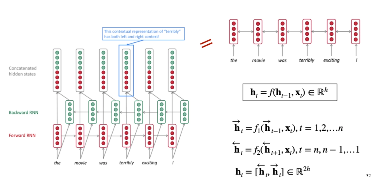
Bidirectional RNNs capture both past and future context by processing sequences in both directions.
•
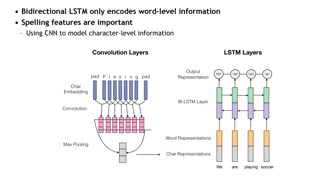
Character-level CNNs combined with BiLSTMs improve representation by capturing morphological features.
•
Structured models like CRFs explicitly model dependencies between output tags and capture global sequence consistency.
•
CRFs use global normalization over entire sequences, while MEMMs use local normalization, making CRFs more effective for sequence labeling.
•
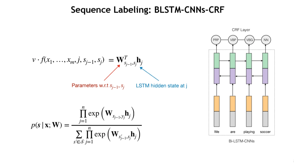
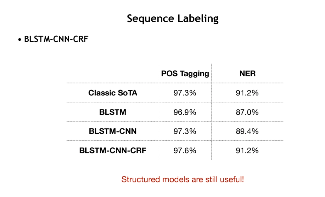
BiLSTM-CNN-CRF architecture combines neural feature extraction with structured prediction for state-of-the-art sequence labeling performance.

Structured Prediction & Sequence Labeling
Structured Prediction
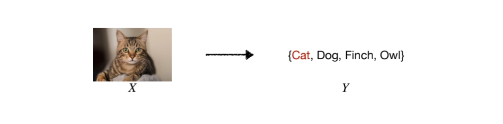
•
Y consists of multiple components Y = {y1, y2, y3}
•
(Strong) correlations between output components
◦
e.g. words in one sentence
•
Exponential output space
•
Types of Sequence Labeling
◦
Part-of-speach Tagging
◦
Named Entity Recoginition
◦
Information Extraction
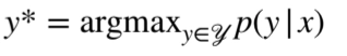
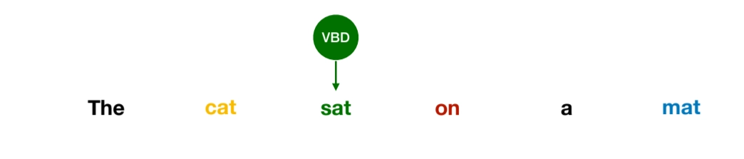
Part-of Speeach (POS) Tagging
•
Word classes or syntatic categories
•
Reveal useful information about the syntatic role of a word
◦
Different words have different syntatic functions
◦
It’s DIsambiguation task
▪
Each word might have different senses/functions
◦
There are 45 tags in English (Penn Tree Bank Tagset)
•
POS Tagging has not solved yet
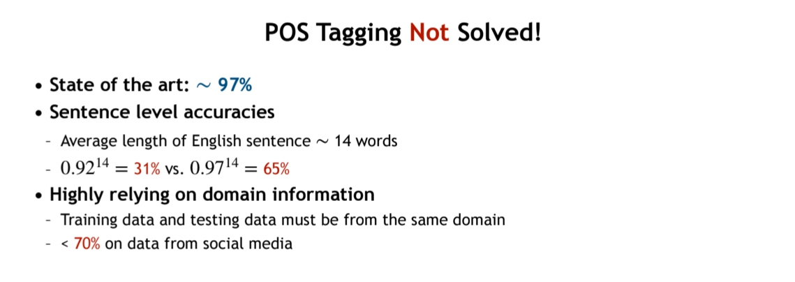
•
In POS tagging, we can observe that
1.
The function (or POS) of a word depends on its context
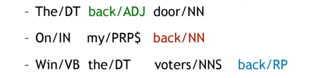
2.
Certain POS combinations are extremely unlikely

3.
Better to make predictions on entire sentences instead of individual words
•
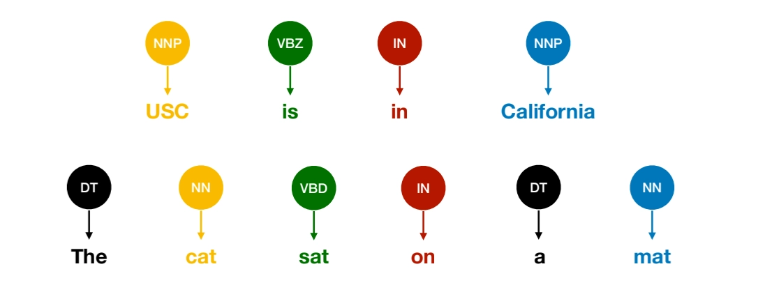
Do we need structured models if the feature representations of the input sentence is perfect?
◦
In theory, no. If the feature representation of each word perfectly captures all contextual information in the sentence, we could predict each tag independently. In that case, modeling the joint probability of the tag sequence would not be necessary.
◦
However, in practice, a word’s correct tag often depends not only on the input words but also on neighboring tags. For example, certain POS tags are more likely to follow specific tags (e.g., a determiner is often followed by a noun).
◦
Therefore, we cannot safely assume that tag predictions are fully independent.
•
So, we need structured models that
◦
explicitly model dependencies between output tags,
◦
capture global consistency across the entire sequence,
◦
and learn transition patterns such as
•
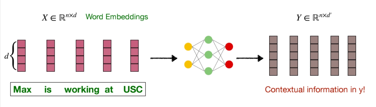
One feature vector for each word
Recurrent Neural Network (RNN)
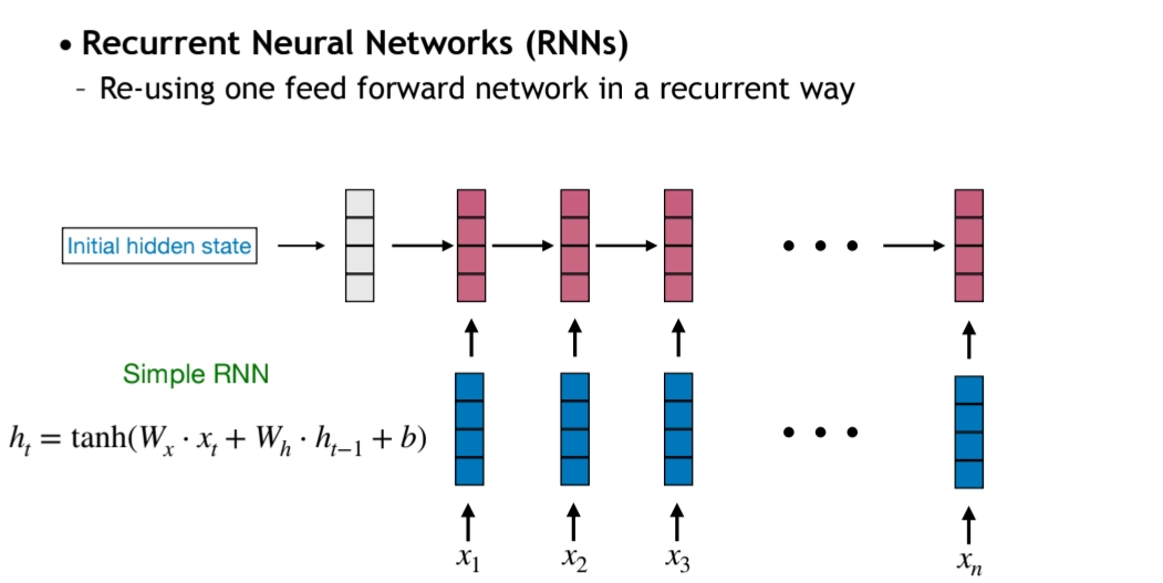
•
Problems of Simple RNN
1.
No future contexts
•
Future information is important for sequence labeling tasks
2.
Inefficient (Sequential Computation)
3.
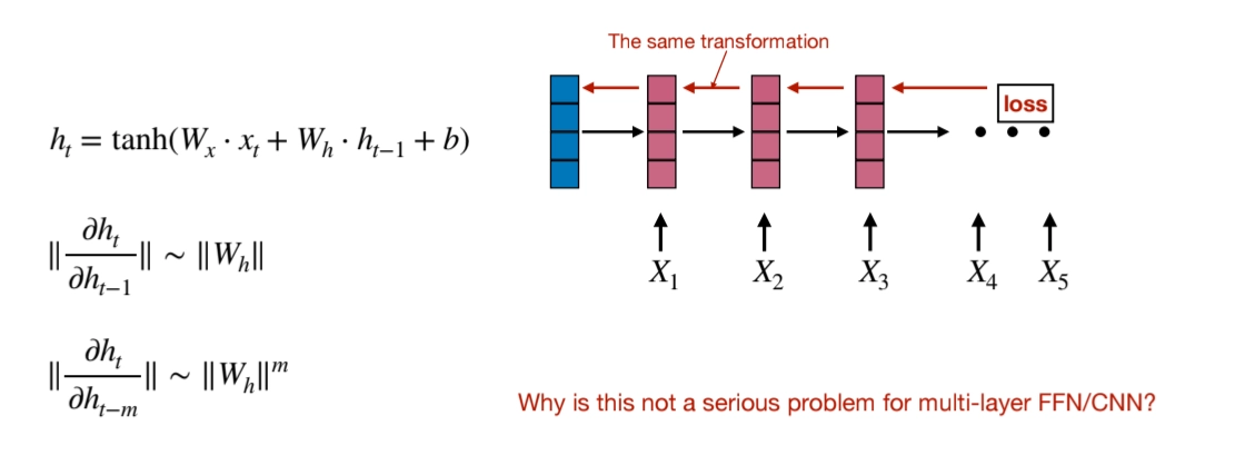
Hard to train → Gradient Varnishing/ Exploding
•
Why is this not a serious problem for multi-layer FFN/CNN?
1.
No repeated weight multiplication: In RNNs, the same weight matrix is multiplied repeatedly across many time steps, which can exponentially amplify or diminish gradients. In FFNs/CNNs, each layer has different weights, so this compounding effect doesn't occur in the same way.
2.
Skip connections and normalization: Modern architectures like ResNet use skip connections and batch normalization, which help gradients flow more smoothly through deep networks.
3.
Independent layer computations: Each layer's computation is independent of previous time steps, making the gradient flow more stable compared to the temporal dependencies in RNNs.
4.
Limited size of hidden states (Memory Cost)
Bidirectional RNNs (Solving Prob#1)
Advanced RNN Variants (Soving Prob#3)
LSTMs for Sequence Labeling
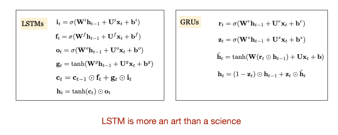
LSTM: Long Short-Term Memory
•
Key idea of LSTM
◦
LSTM introduces a separate cell state that acts as long-term memory.
◦
Information can flow through this cell state with minimal modification.
◦
Gates control what to forget, what to add, and what to output.
•
Input gate: controls how much new information is written into memory. It decides which parts of the candidate vector should be stored.
◦
•
Forget gate: controls how much of the previous memory should be kept. If the value is close to 0, information is forgotten. If it is close to 1, information is preserved.
◦
•
Candidate vector: a temporary vector containing new information computed from the current input and previous hidden state. It is combined with the input gate before being added to memory.
◦
•
Cell state update: the new cell state is formed by keeping part of the old memory (controlled by the forget gate) and adding selected new information (controlled by the input gate).
◦
•
Output gate: controls how much of the internal memory is exposed as the hidden state. Not all stored information needs to be shown at every time step.
◦
•
Final hidden state: the hidden state is a filtered version of the cell state. It is passed to the next time step or next layer.
◦
•
Why LSTM works better
◦
the additive memory update helps reduce the vanishing gradient problem.
◦
The gating mechanism allows the model to selectively remember important information. This enables learning long-range dependencies in text, speech, and time-series data.
•
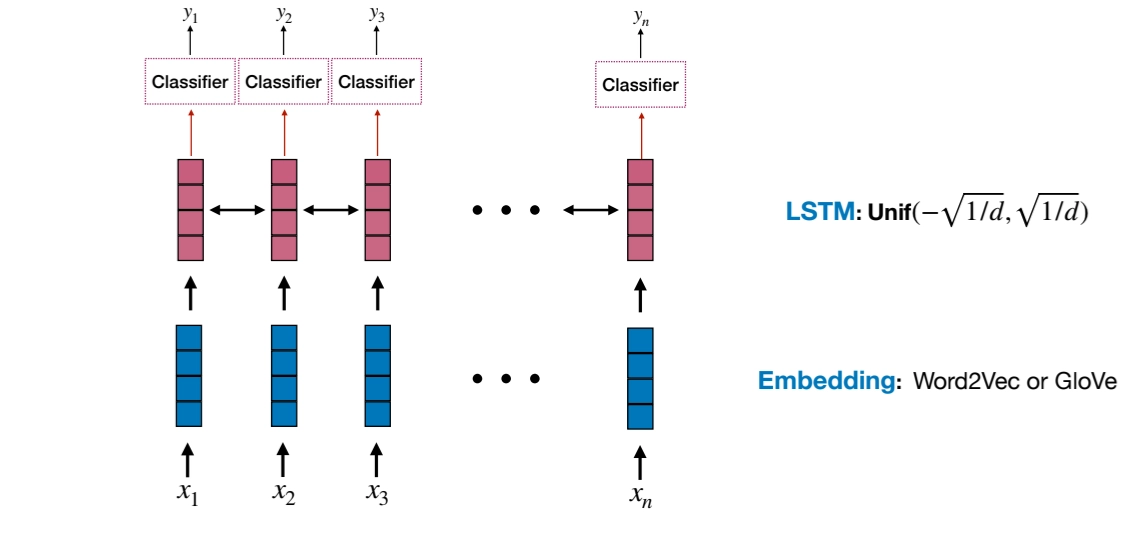
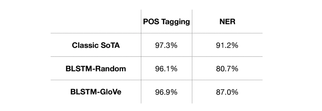
For Sequence Labeling, a simple bidirectional LSTM model is not good enough
Bidirctional LSTMs + CNNs for Sequnce Labeling
BiLSTM-CNNs-CRF for Sequence Labeling

•
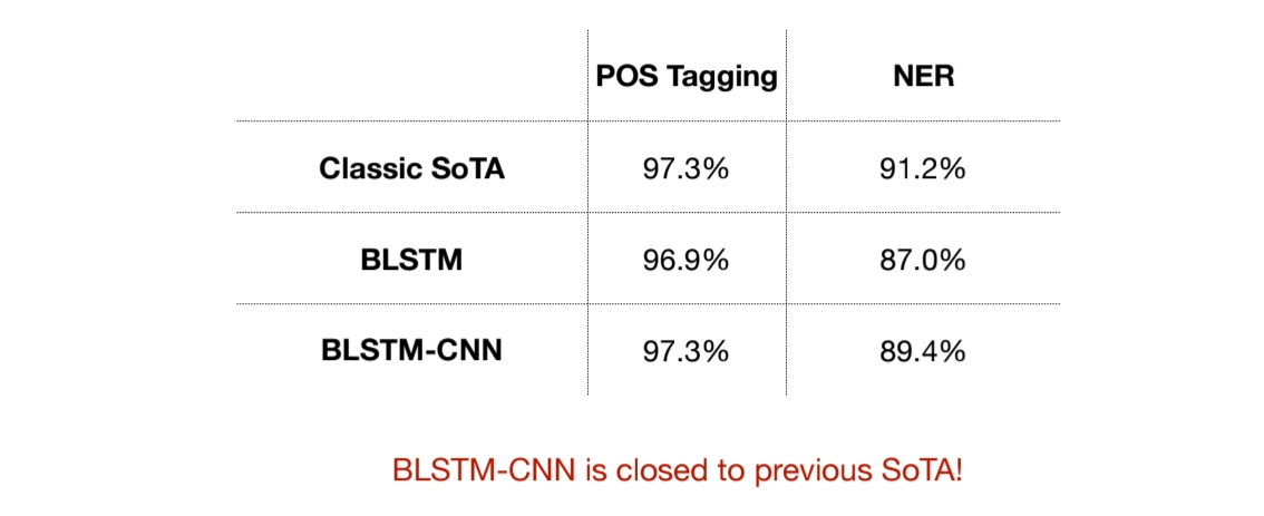
BiLSTM + Char-level CNN is not strong enough → How about combining structured models with LSTM?
•
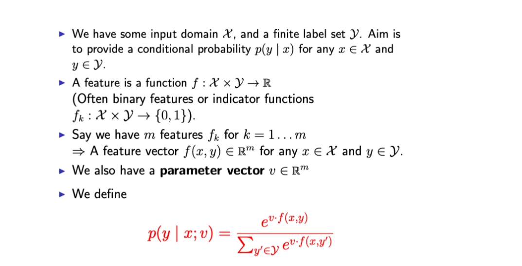
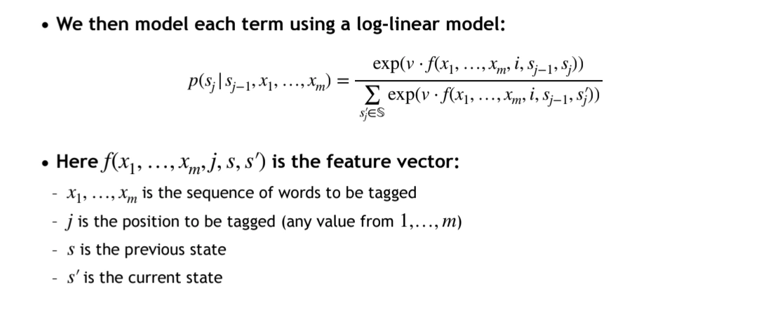
Log-Linear Models

◦
What is features in Log-Linear Models
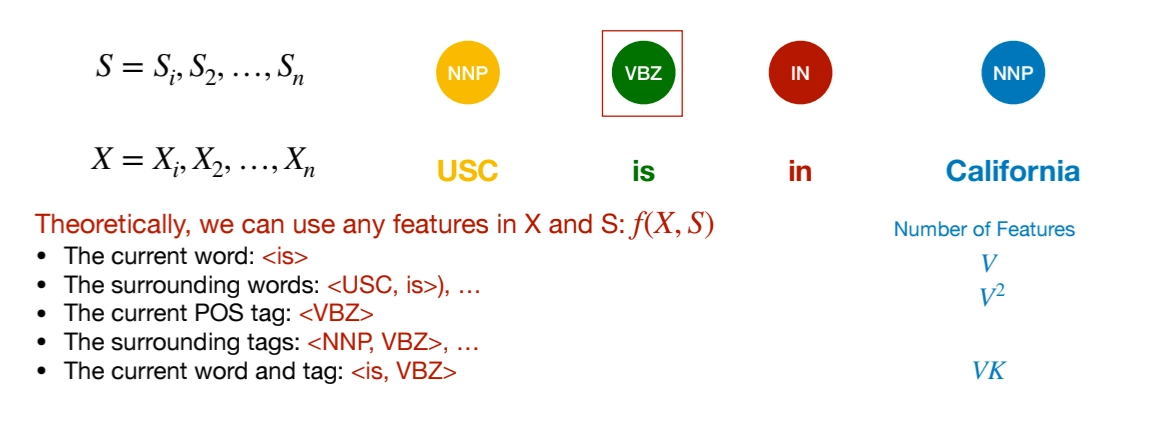
But there is feature sparsity problem. As we add richer features (bigrams, word–tag pairs, etc.), the feature space explodes.
▪
Most features are never observed
▪
Most feature vectors are extremely sparse
▪
We don’t have enough data to estimate all weights reliably
◦
We need independence assumptions to compute the nominator

◦
The denominator (normalizer) sums over all possible outputs.
▪
To compute that denominator efficiently, we need independence assumptions.
1.
Maximum Entropy Markov Models (MEMMs)
•
for the independence assumption, use Markov Property (Markov Assumption)
In the denominator we are only summing over all possible tags for the current position j. → locally calculation
If the tag set size is K, then: the denominator costs O(K)
•
MEMMs has flexibility on combination of features
2.
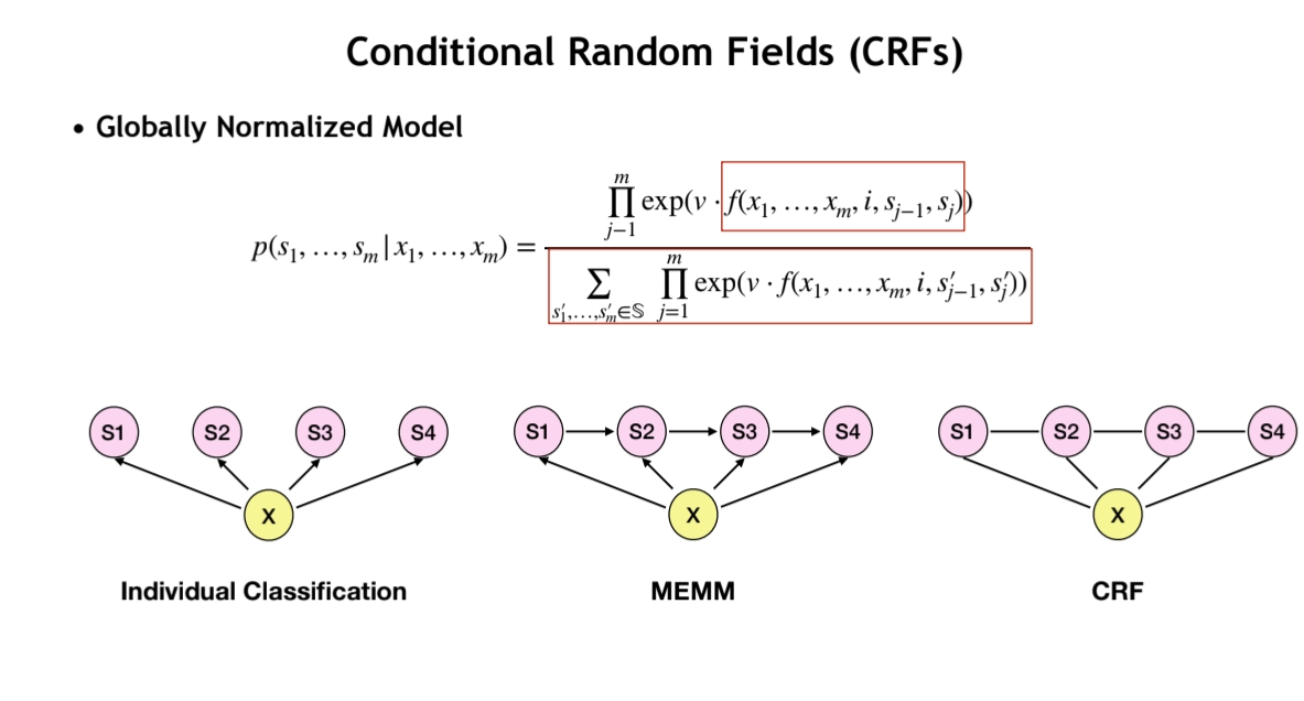
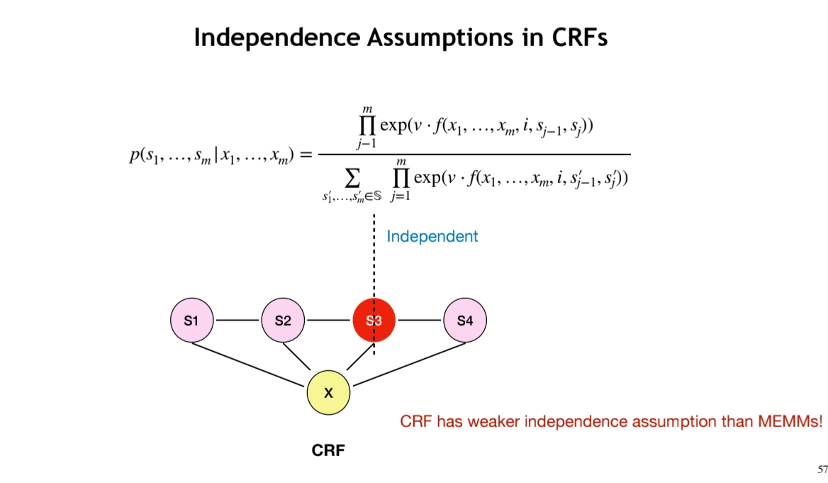
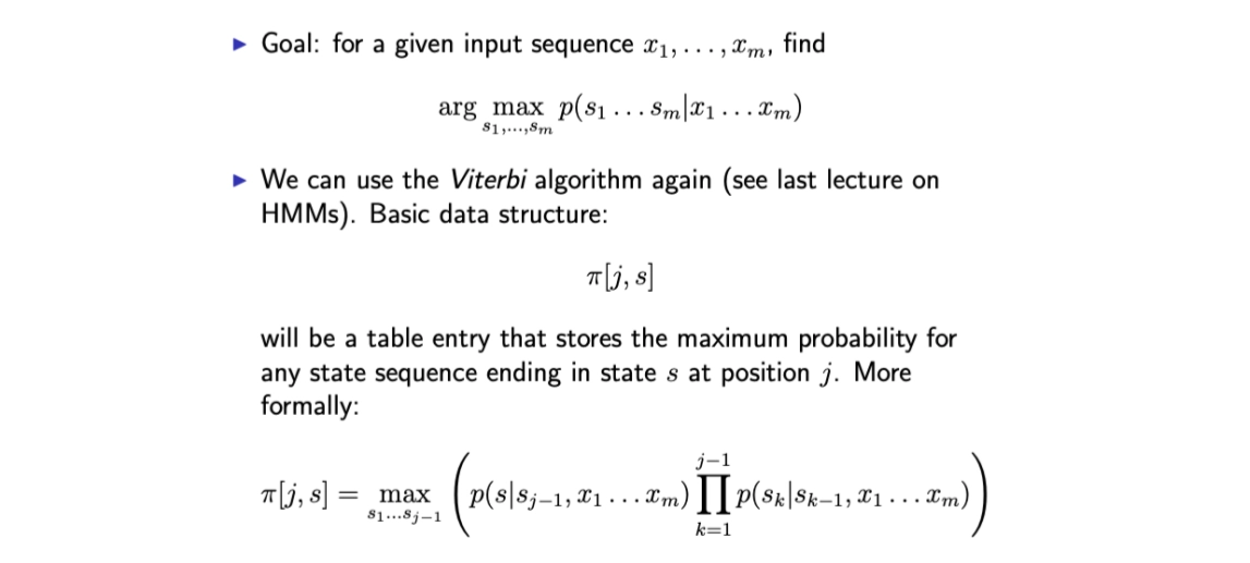
Conditional Random Fields (CRFs)
•
It’s Globally Nomalized Model
◦
CRFs have weaker independence assumption than MEMMs
•
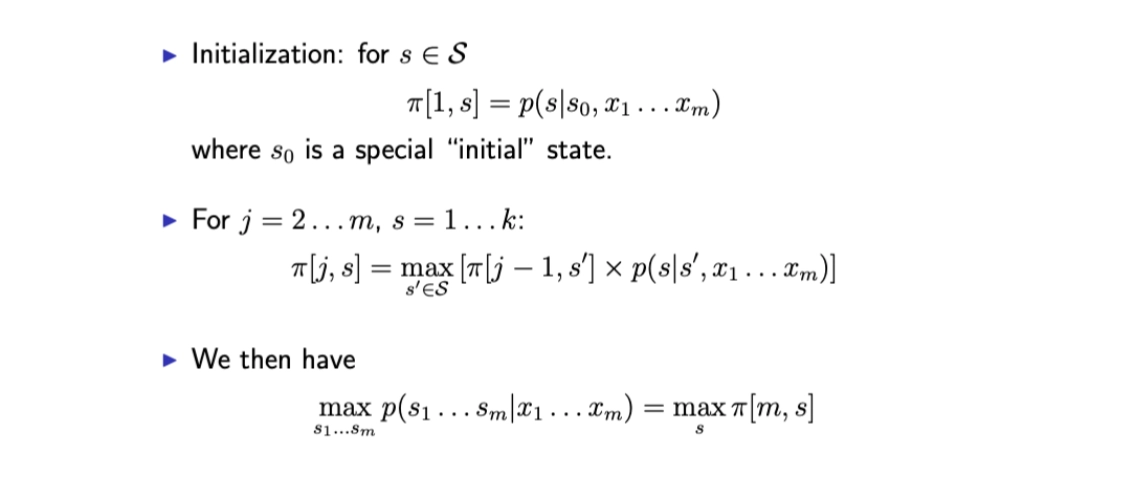
How to compute?
◦
Viterbi Algorithm
•
BLSTM-CNN-CRF
NLP - Lecture Summary
Search