
•
NLP systems consist of feature extraction and machine learning components, with deep learning replacing manual feature engineering
•
Text classification can be approached through generative methods (Naive Bayes) or discriminative methods (Logistic Regression, SVM)
•
Naive Bayes assumes conditional independence of words given labels and uses Bayes Rule to compute P(y|x)
•
Laplace smoothing addresses zero probability problems by adding pseudocounts; log space prevents numerical underflow
•
Logistic Regression learns weights for features to compute scores, converting them to probabilities via sigmoid function
•
Training optimizes parameters by maximizing log-likelihood (minimizing cross-entropy loss) using gradient descent
•
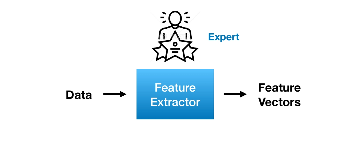
Feature extraction methods include unigram counts, which are simple but lose word order information
•
SVM provides an alternative discriminative approach for training linear classifiers
NLP System Pipeline
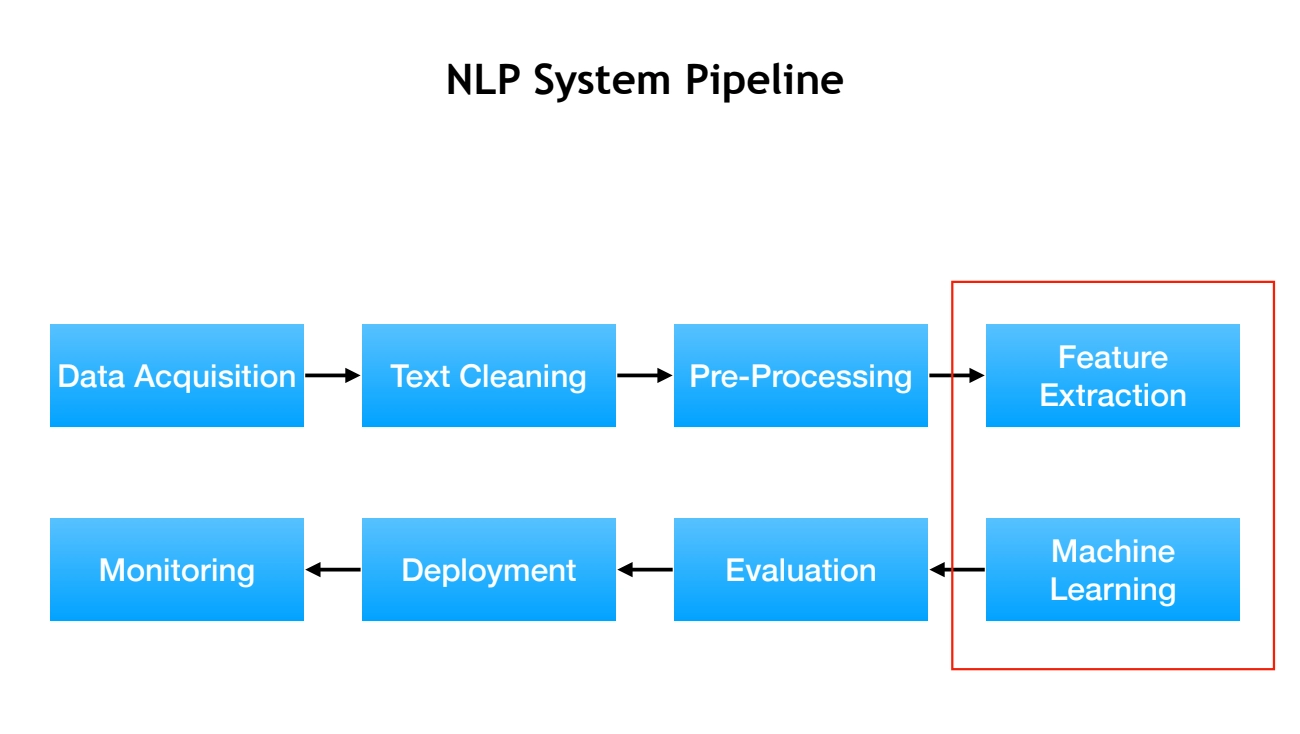
Feature Extraction
•
For example,
◦
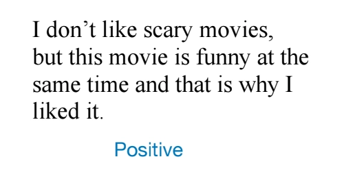
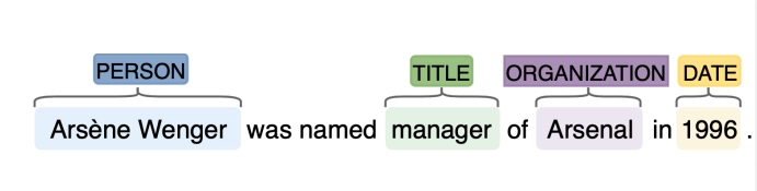
Sentiment Analysis
◦
Named Entity Recognition
•
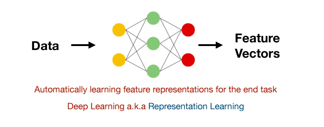
Limitations of Expert System
◦
Different expertise for different tasks
◦
Expertise is not transferrable across tasks, languages, and domains
◦
⇒ solution is Deep Learning a.k.a Representation Leanrning
Machine Learning
•
Classification
◦
Linear Classifier / Logistic Regression / SVM
•
Structured Predition
◦
Sequence Labeling / CNN / RNN / LSTM
•
Machine Translation
◦
Seq2seq generation
◦
Transformer
•
Language Modeling
◦
Pre-training
◦
Post-training, RL
Text Classification Methods
•
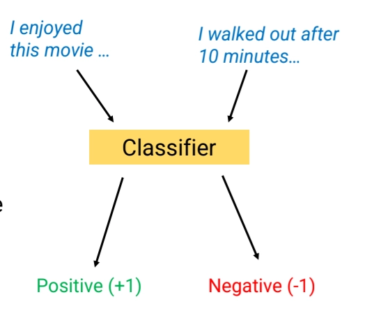
Our goal: Build a sustem that predicts whether a document X, a input, belongs to one of C classes
•
Some text classification problems include:
◦
Sentiment analysis
◦
Hate speech detection
◦
Authorship analysis
•
How to build a Text Classifier
Assume we have training data where i ranges from 1 to
Each input is a document → Documents can have different numbers of words
Each training example has corresponding label
Pre-Processing
•
Goal: Convert data into a standardized form that our models can easily ingest
•
Tokenization: splitting the text into units for processing
◦
e.g. Removing extra spaces, Removing “unhelpful” text, Splitting punctuation
•
Other optional operations include
◦
Contracting and standardizing (e.g. won’t → will not)
◦
Converting capital letters to lowercase (His → his)
◦
Removing stopwords (a, the, about …)
◦
Stemming or lemmatization (e.g. running → run; poorly → poor)
•
Why we do standadization? It helps Generalization
◦
But, as a trade-off: we lose information
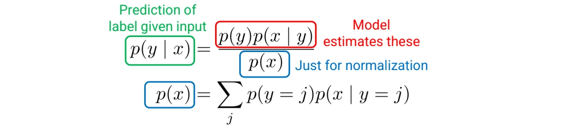
Naive Bayes
•
We model
1.
: For each label . what is the probability of y occurring?
2.
: For each label y, what corresponding ’s are likely to appear?
Modeling Naive Bayes
•
using Bayes Rules,
We can predict the class by choosing the label that maximizes :
1.
Modeling
•
modeling is easy: just count how often each y appears
: the # of possible classes
Our model learn model parameter for each possible
◦
Learning:
▪
: # of training examples
▪
: how often y=j in training data
2.
Modeling
→ In this part, we are using Naive Bayes Method
•
Idea: Make a simplifying assumption about p(x|y) to make it possible to estimate
•
Assumption: Each word of the co x is conditionally independent given label y:
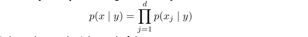
◦
Note: This assumption does not have to be true, just has to be “close enough” so that classifier makes reasonable predictions
•
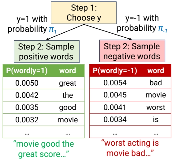
Navie Bayes posits its won probabilistic story about how the data was generated
•
Process
1.
Each was sampled from the prior distribution
2.
Each word in was ampled independently from the word distribution for label
•
Why is the Naive Bayes Assumption OK?
Naïve Bayes assumes:
Once the label y is chosen, each word is generated independently.
So it assumes something like:
positive document generation:
great the movie good score great the ...
negative document generation:
bad worst movie is terrible worst bad ...
Plain Text
복사
This is unrealistic. Real sentences are:
"the movie was great"
"the acting was terrible"
Plain Text
복사
Words clearly depend on each other.
For example:
◦
"New" → likely followed by "York"
◦
"machine" → likely followed by "learning"
Not independent.
So clearly, Naïve Bayes assumption is wrong.
But, Why is the Naive Bayes Assumption OK?
since w e don’t need exact probabilities. We only need the correct class to have higher probability.
For example,
Learning with Naive Bayes
•
How to learn? Just count occurences of w
◦
Note: this formula has a flaw, we will fix it soon
•
Model learns parameter
◦
Total of parameters to learn
▪
denote the set of words in the dictionary
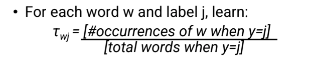
See the below example,
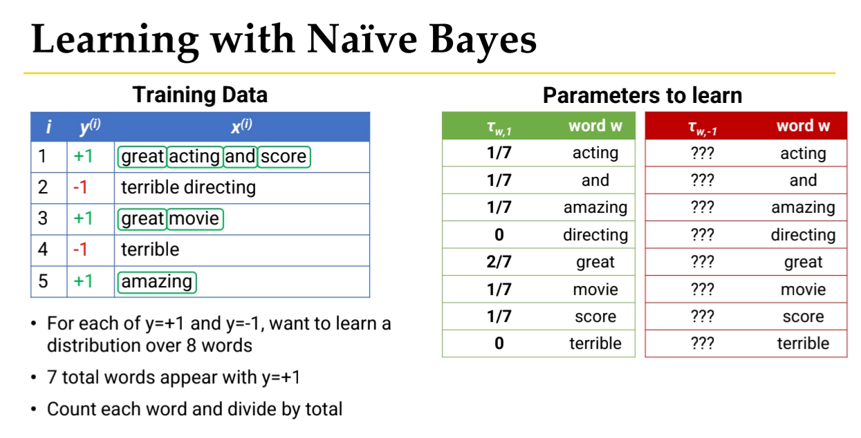
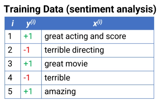
1.
We begin with labeled text documents:
i | y(i) | x(i) |
1 | +1 | great acting and score |
2 | -1 | terrible directing |
3 | +1 | great movie |
4 | -1 | terrible |
5 | +1 | amazing |
Where:
•
x(i) = document (sequence of words)
•
y(i) = label
◦
+1 → positive
◦
−1 → negative
Our goal is to learn:
These are called the likelihood parameters and are denoted:
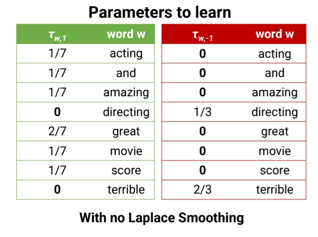
In Positive documents:
great acting and score
great movie
amazing
Plain Text
복사
Count each word:
word | count |
great | 2 |
acting | 1 |
and | 1 |
score | 1 |
movie | 1 |
amazing | 1 |
directing | 0 |
terrible | 0 |
Total words in positive class: 7
2.
Let’s convert Counts into Probabilities
Formula:
P(w∣y=+1)=count of w in positive docstotal positive wordsP(w \mid y=+1) =
\frac{\text{count of w in positive docs}}{\text{total positive words}}
P(w∣y=+1)=total positive wordscount of w in positive docs
So:
word | probability |
acting | 1/7 |
and | 1/7 |
amazing | 1/7 |
directing | 0 |
great | 2/7 |
movie | 1/7 |
score | 1/7 |
terrible | 0 |
This produces the green table in the image.
Same in Negative examples.
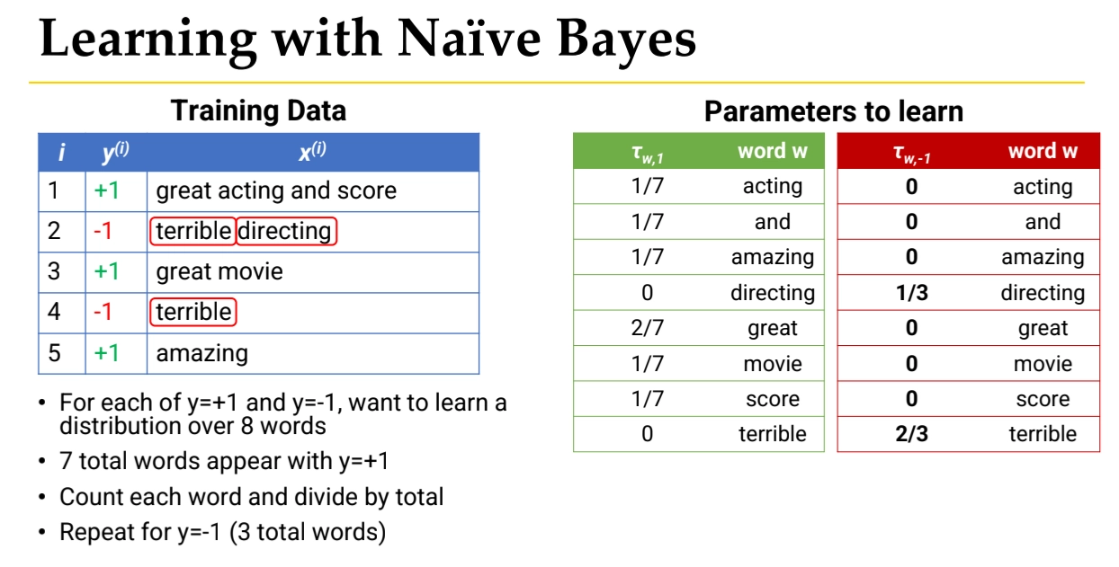
Predicting with Naive Bayes
Problems of Naive Bayes
1.
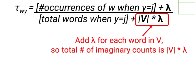
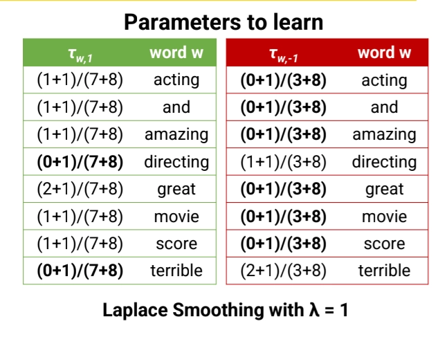
Too Many Zeros → Laplace Smmothing
What if both and have zero value?
By Bayes Rule,
But the model assign probability of 0 to many (word, label) pairs.
•
Solution: Laplace Smoothing
is a new hyperparameter
◦
Imagine that every (word, label) pair was seem an additional times
2.
Numerical Underflow → Using Log Space
Given long test example, the probability goes underflow.
Since multiplying many small numbers results in numerical underflow, and the result is so small that it becomes 0
•
Solution: using log
Summary
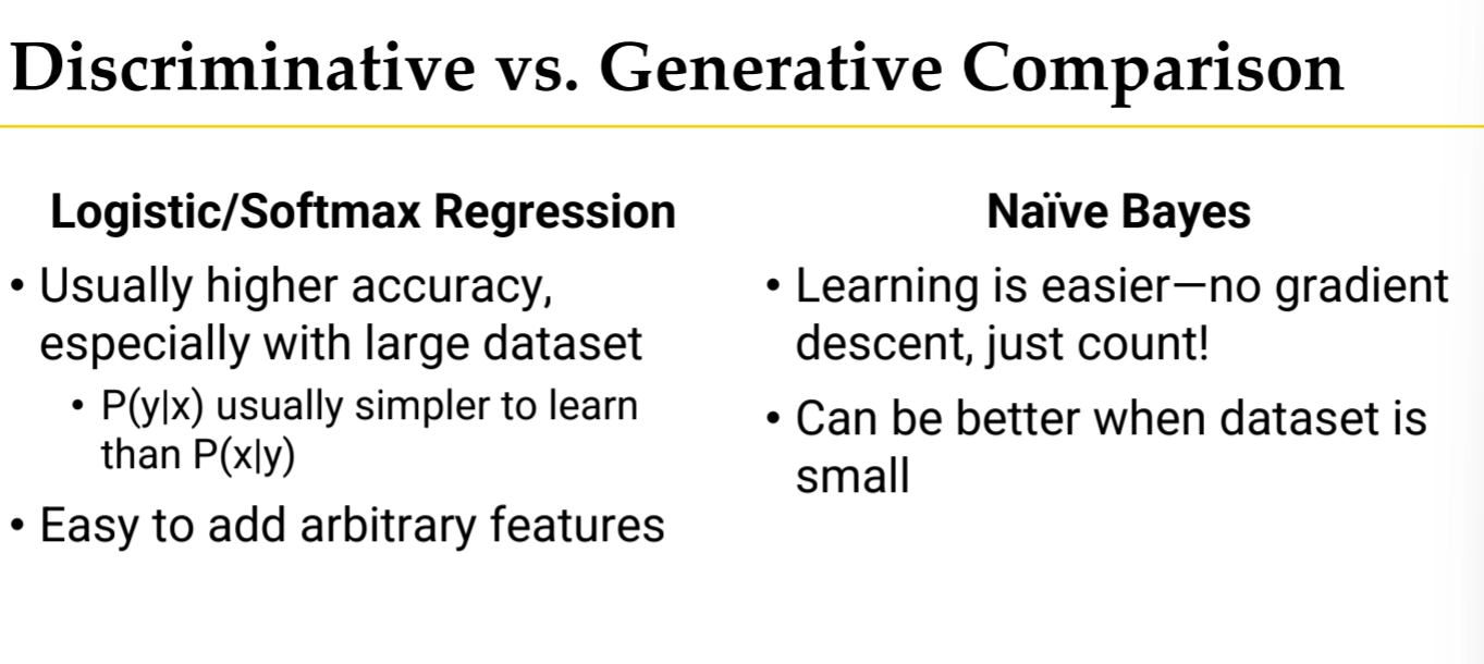
Logistic & Softmax Regression
•
First decide on a formula we will use to make predictions
◦
Formula contains some numerical parameters which determine its output
◦
Optimize the parameters so that we make good predictions on the training data
◦
Discriminative: Focuses only on discriminating positives & nagatives
▪
vs Naive Bayes (Generative Approach) : it models the entire process of generating (x,y)
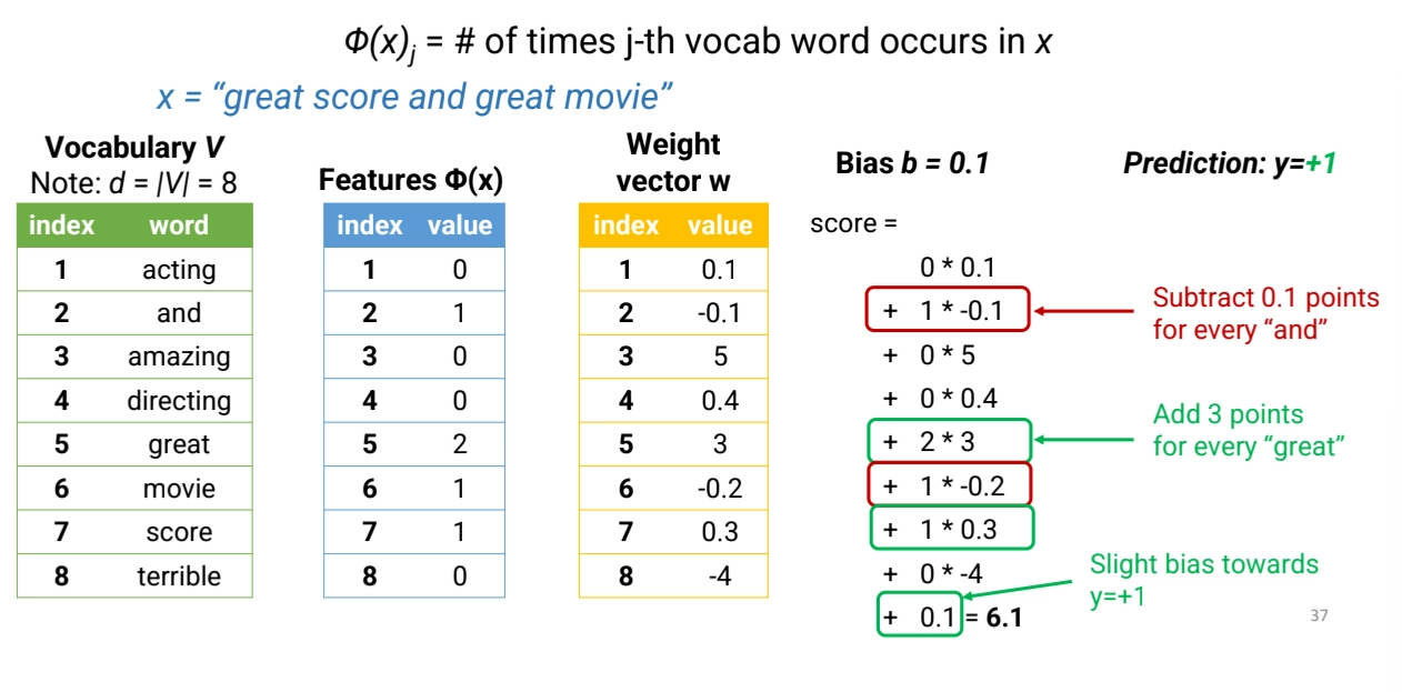
Predicting with Logistic Regression
1.
Convert the document x to a vector of features of length
2.
Choose (in advance) a weight vector w of length d and a bias b
•
so, our params are w, d, b
3.
Compute a score as follows:
Note: this is a linear model b/c score is linear function of features
4.
Predict if score > 0, otherwise
Feature Extraction Phase
•
Example: Unigram Count Features
◦
First construct a vocab: set of all words in the training data
◦
Unigram Count Features
▪
Pros
•
We can learn how each word influences label
•
Very simple
•
Can work reasonably well for some tasks
•
# of params we have to learn is not that large
▪
Cons
•
We lose all information about order of words
•
Doesn’t really captrue what the sentence means
Machine Learning Phase
•
How to choose w & b?
◦
Idea: Optimize w & b to ensure our predictions are accurate on the training data
◦
What does "good" mean?
▪
Good: make correct predictions
▪
Better: make confidently correct predictions
•
Score should be very high when y = +1. Score should be very low when y = -1
◦
Our approach: convert scores to probabilities and maximize the probability of the correct answer
cf) Sigmoid Function
•
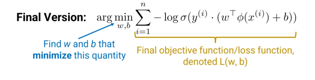
Objective Function
◦
We want to optimize this objective function with respect to w & b
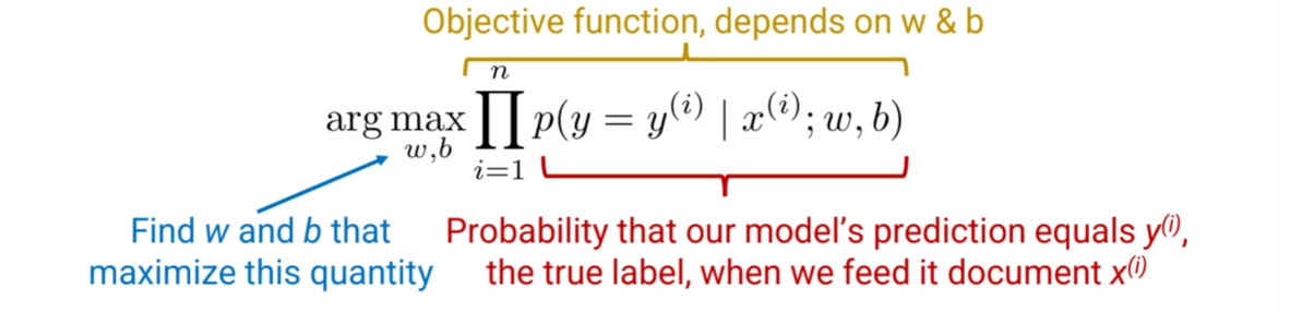
◦
for binary classification,
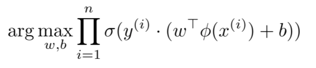
And tkae log and negate
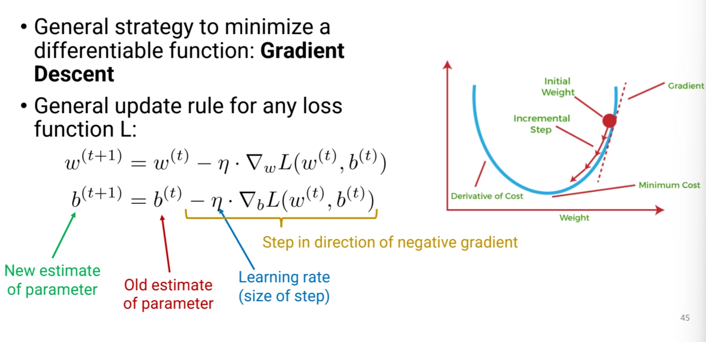
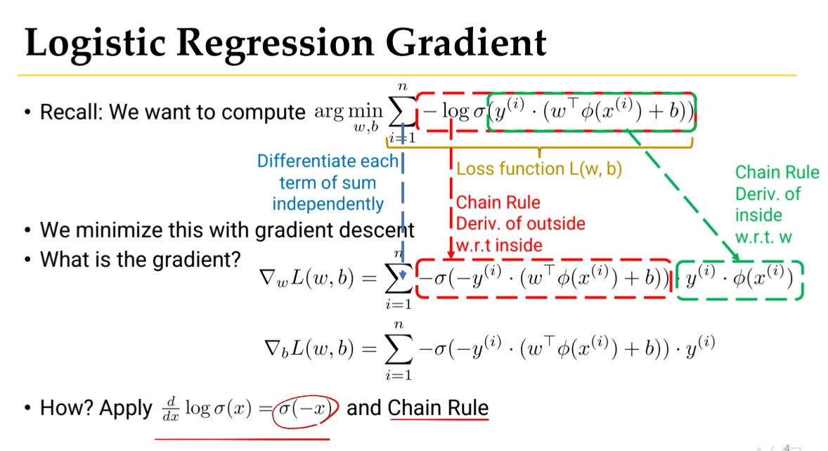
•
Optimization
◦
Using Gradient Descent
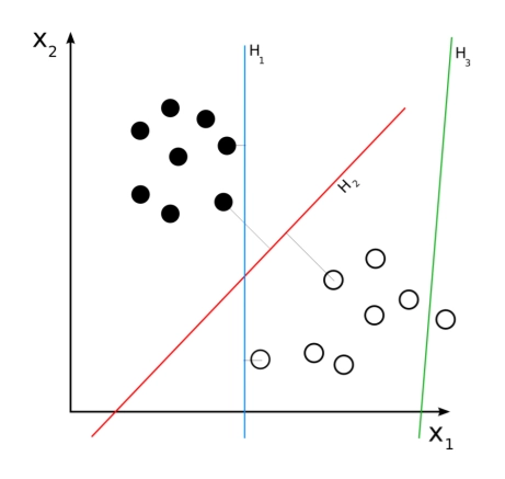
Support Vector Machines (SVM)
•
This is an another method for training a linear classifier
◦
Also learns w, b
•
Intuition: Find a separating hyperplane with large margin
•
Location of hyperplane winds up depending on support vectors
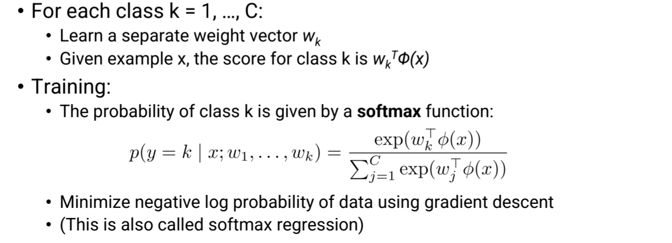
Multi-class / Multinomial Logistic Regression
•
what if we have C > 2 classes?
◦
using Softmax Function
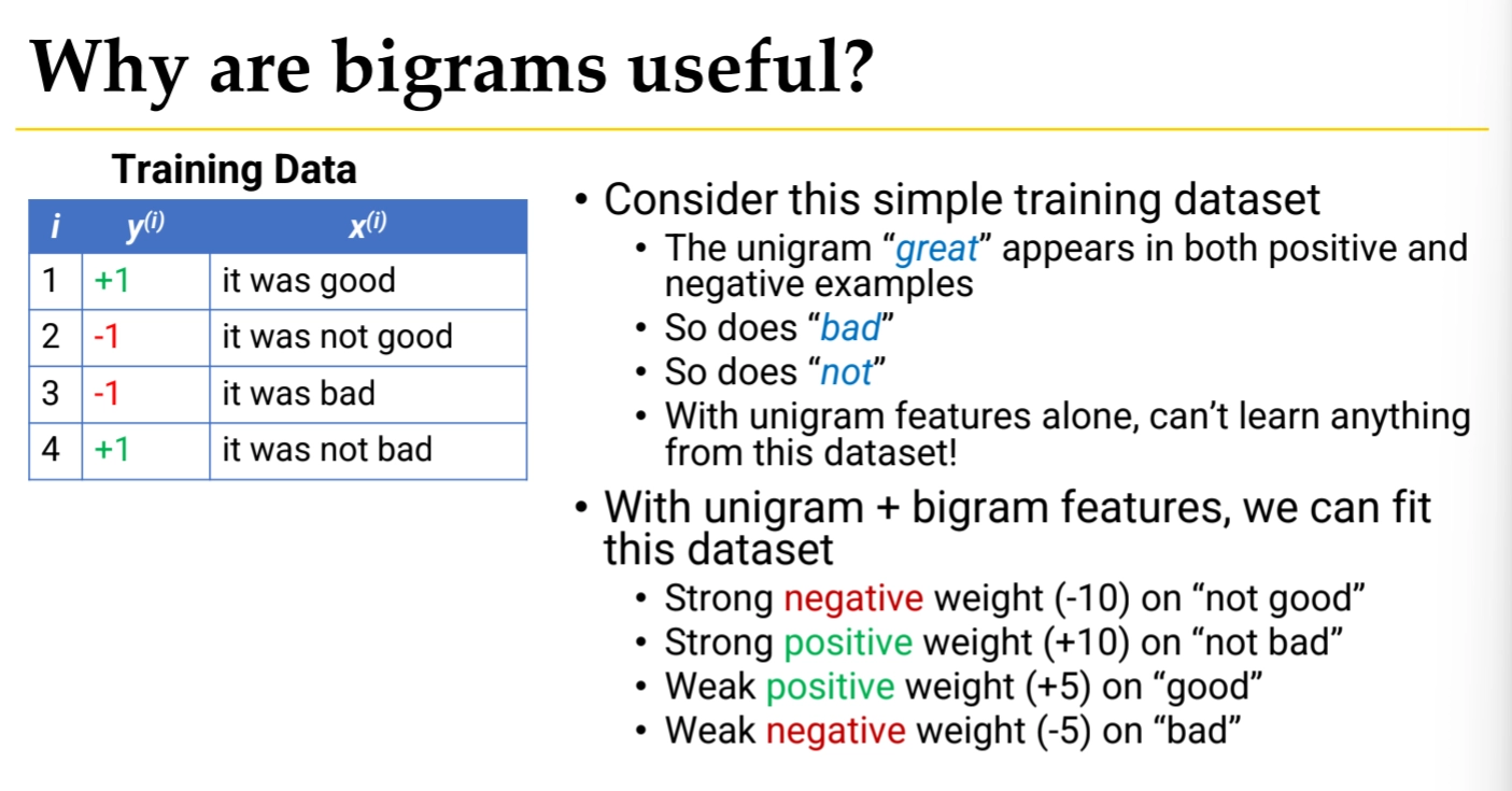
Biagram
•
Bigram = pair of consecutive words
A bigram is simply two consecutive words that appear together. For example, in "great movie," the bigram is ["great", "movie"].
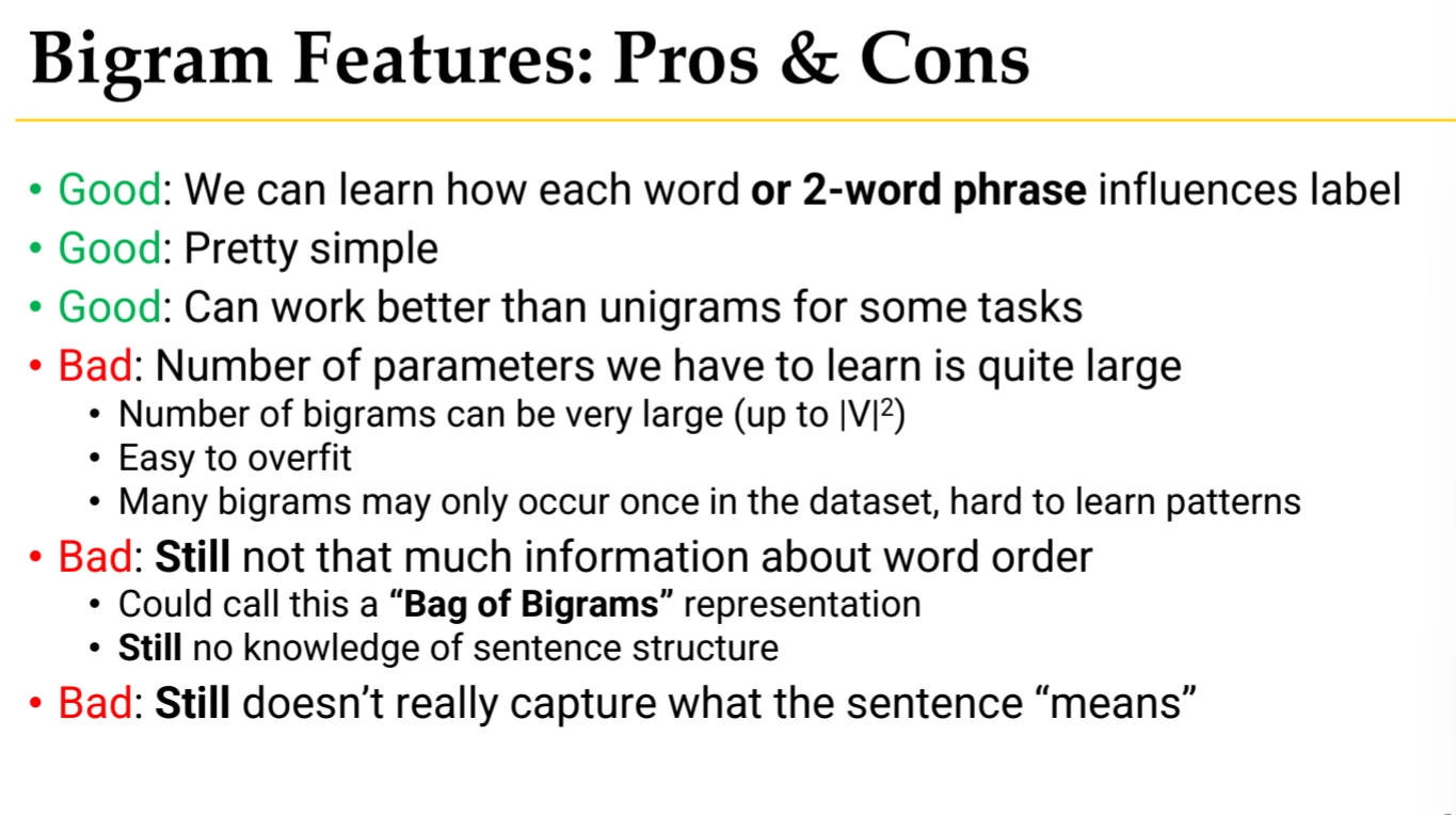
When you use bigram features, you create a separate feature for each possible pair of words. If your vocabulary has |V| words, the number of possible bigrams is |V|² (vocabulary size squared). This means if you have 10,000 words in your vocabulary, you'd have 100 million possible bigram features.
For each bigram feature, the model learns a separate weight parameter. This allows the model to capture patterns like:
◦
"not good" (negative sentiment) vs "very good" (positive sentiment)
◦
"highly recommend" (strong positive) vs "do not" (likely negative)
In practice, you typically use both unigram and bigram features together. This gives your model:
◦
Unigrams: Individual word importance (e.g., "terrible" is negative)
◦
Bigrams: Word order and context (e.g., "not terrible" changes the meaning)
◦
Pros and cons
Discriminative vs. Generative Comparison
Model Evaluation
Our goal is always to build a classifier that can calssify any document
•
Model will overfit to the training data
•
We need to test generalization to unseen examples
•
Split dataset into three parts
◦
Training set: Train the model
◦
Development set (Validation set): Select hyperparams
◦
Test set : evaluate final model’s performance
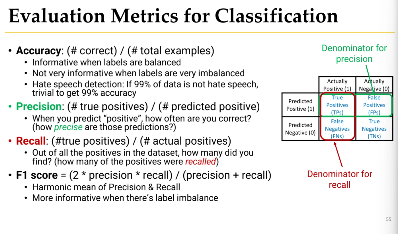
Evaluation Metrics
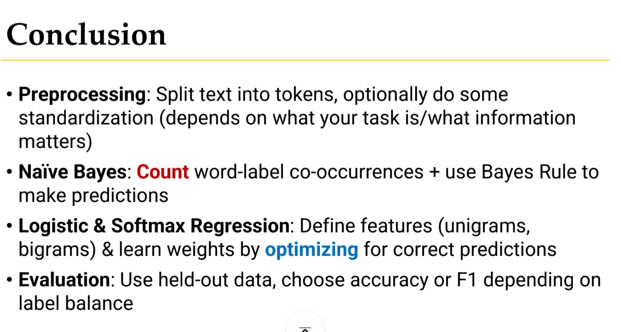
Conclusion
NLP - Lecture Summary
Search